







Magnetic Coupling Synchronous Torque Lock & Extreme Temperature Anti-Demagnetization Design
Abstract
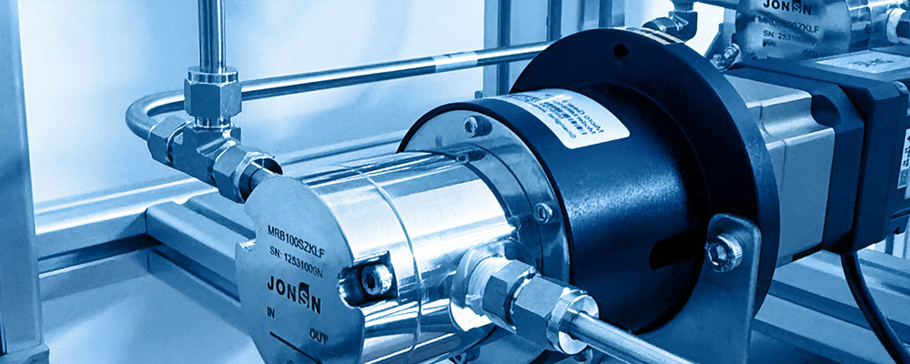
Magnetic drives use the paradigm of "static seal replacing dynamic seal" to completely eliminate the leakage path at the shaft seal of centrifugal and gear pumps, becoming a mandatory technical route for semiconductor wet chemicals, strong-corrosion media, high-purity and hazardous-media transport. Its core is a deceptively simple yet highly coupled physical system: between the outer magnetic rotor and the inner magnetic rotor there sits a layer of non-magnetic containment can, with the magnetic flux lines of NdFeB permanent magnets penetrating through to achieve contactless torque transmission.
The fatal vulnerability of this system lies in a chained failure link: when the load torque exceeds the magnetic coupling's maximum synchronous torque, the inner and outer rotors experience "pull-out"; after pull-out, the rotors move at large slip relative to each other, inducing eddy currents inside the containment can; the slip power heats the can to several hundred degrees within tens of seconds; the rising temperature simultaneously decays the NdFeB remanence B_r and intrinsic coercivity H_cJ; once the working point drops below the knee point of the demagnetisation curve, irreversible demagnetisation occurs, the magnetic coupling torque permanently decreases, and the pump fails completely. Every link in this chain amplifies the next, forming a typical positive-feedback thermal runaway.
This white paper takes a 50-bar (5.0 MPa) pressure-difference shock as the design-driving duty and a temperature envelope of −196 °C - +200 °C, establishes and solves the complete mathematical model coupling four fields — magnetic-circuit, eddy-current, thermal and mechanical — and delivers a re-computable, verifiable engineering methodology:
1Model 1 (magnetic-circuit penetration): The permanent-magnet equivalent magnetic circuit and permeance-coefficient P_c model are built, and the influence of the non-magnetic containment can is analysed. Quantitative proof is given: in the typical magnetic-pump slip-frequency range (50 – 600 Hz), the skin depth of a Hastelloy containment can reaches 47.7 mm, i.e. 21.7× its wall thickness (2.2 mm); the magnetic Reynolds number R_m = 0.123 << 1, and the magnetic-flux penetration rate reaches 99.25 %. This mathematically validates the engineering intuition that "magnetic flux lines can effectively penetrate a non-magnetic containment can", including its boundary conditions.
2Model 2 (synchronous torque): The torque–torque-angle characteristic T(Δθ) = T_max·sin(m·Δθ) and the analytical expression for maximum synchronous torque are given; the pull-out dynamics of magnetic coupling are shown to be completely isomorphic to the swing equation of a synchronous generator, so the Equal-Area Criterion of power systems can be transplanted directly as the pull-out criterion. Three tiers of "torque lock" are defined — static lock, dynamic lock, thermal lock — with quantitative criteria for each.
3Model 3 (slip-induced heat): The exact expression for slip power P_slip = T_async·Δω is derived from energy conservation, together with the Kloss formula describing asynchronous torque. The worked example shows that the 50-bar, 2.4 mL/rev magnetic gear pump under full-slip pull-out at 1450 r/min has slip power up to 1 012 W; the metal containment can (Hastelloy C276, t = 2.2 mm) heats at 8.65 K/s, reaching demagnetisation temperature in only -21 s — an extremely narrow protection window. Switching to a SiC ceramic containment can drops the eddy-current distribution coefficient from 0.85 to 0.02, reducing the heating rate to 0.54 K/s and extending the protection window 16× to 5.6 minutes.
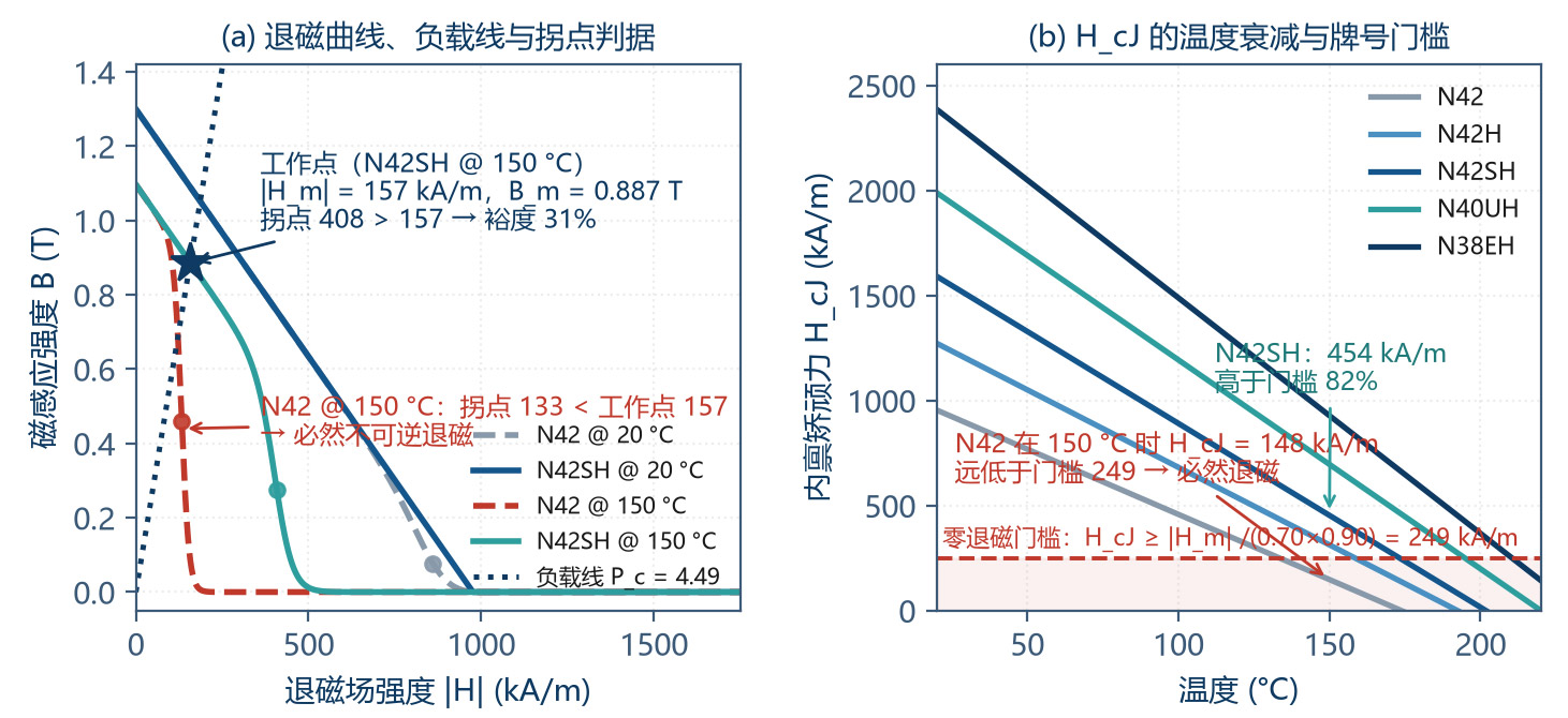
4Model 4 (anti-demagnetisation): A knee-point demagnetisation criterion with temperature effect is established, |H_m| ≤ 0.7·H_k(T), and the minimum permeance-coefficient method is given. A key quantitative finding: in a magnetic circuit with P_c = 3.37, the ordinary grade N42 at 150 °C has H_cJ decayed to 148 kA/m while the working-point field strength reaches 184 kA/m — far beyond the knee point — guaranteeing irreversible demagnetisation; N42SH at the same temperature retains H_cJ = 454 kA/m with 31 % margin. Meanwhile, the Grain Boundary Diffusion (GBD) technique is shown to exchange 2 – 5 % B_r loss for 30 – 60 % H_cJ gain — the highest cost-performance anti-demagnetisation measure.
Cryogenic trap: The false impression of "better performance" caused by NdFeB B_r rising at low temperature (-+26 % at −196 °C), the spin-reorientation phenomenon near −138 °C, and the cracking risk induced by anisotropic thermal expansion are pointed out, with the material-selection rule that Sm₂Co₁₇ is preferred below −60 °C.
Building on the above models, this paper proposes a unified solution method for the containment can's "strength–magnetism–eddy current" trilemma (external-pressure buckling check + effective air-gap minimisation + material resistivity optimisation), builds five defence lines (soft start, torque limit, slip detection, temperature monitoring, fast power-off), and provides in Chapter 7 a complete 12-step engineering verification procedure with an all-pass design example.
1 Introduction — Physical Boundary of Leak-Free Transmission
1.1 Three Operating Principles of Magnetic Coupling
The essence of magnetic drive is to convert the mechanical quantity "torque" into the field quantity "magnetic field" crossing the static containment can, then convert it back into mechanical quantity. According to the torque-generation mechanism there are three types:
| Type | Torque Mechanism | Synchronism | Slip | Eddy Heating | Applicable Duty |
|---|---|---|---|---|---|
| Synchronous (PM coupling) | Attraction / repulsion between inner & outer magnetic poles, sustained torque angle by magnetomotive force | Strictly synchronous | Normal = 0 | Harmonic only (0.5 – 2 % of rated) | Most magnetic pumps; fixed-speed & high-efficiency duties |
| Asynchronous (eddy coupling) | Outer-rotor field induces eddy current in copper / aluminium ring; eddy field reacts with original | Asynchronous | 3 – 8 % | High (= slip power) | Soft start, overload protection, speed regulation |
| Hysteresis coupling | Hysteresis-loop area of hysteresis material produces constant torque | Sync or slip | Controllable | Medium | Constant-tension winding, torque limiting |
Table 1-1 CoMParison of the three magnetic-coupling principles
The magnetic pump discussed in this paper belongs to the synchronous type. Understanding this is critical: under normal working the synchronous coupling has zero slip and near-zero eddy-current loss, which is the source of its high efficiency (magnetic-coupling efficiency reaches 98 – 99.5 %); but this is also the root of its fragility — once synchronism is broken the system instantly switches from "near-zero loss" to "full slip-power dissipation".
1.2 Failure Chain — Pull-out → Heat → Demagnetisation → Failure
Field failures of magnetic pumps are rarely abrupt fractures; they are a chained link with a definite temporal scale. Understanding the time constant of each link is the basis for designing the protection system:
| Link | Physical Mechanism | Typical Time Scale | Observable Symptom | Intervenable Means |
|---|---|---|---|---|
| ① Overload / shock | Load torque > maximum synchronous torque T_max | ms – s | Motor current spike, outlet P fluctuation | Soft start, torque limiter, slow-open valve |
| ② Pull-out | Torque angle crosses unstable equilibrium; magnetic poles slip off | 10 – 100 ms | Speed signal decouples from command; abnormal noise | Slip detection, fast power-off |
| ③ Slip-induced heating | Eddy current dissipates slip power at large slip | s – min (metal can 8.65 K/s) | Containment-can outer T rises rapidly | Non-metallic can, temperature interlock |
| ④ Irreversible demagnetisation | Working point falls below demag-curve knee point | Permanent once it occurs | Torque permanently drops, current anomaly | None (only replace magnetic rotor) |
Table 1-2 Four links of the magnetic-coupling failure chain & their time scales
The key feature of this chain is positive feedback: the heat of link ③ raises the magnet temperature, B_r and H_cJ decay, and T_max decreases (T_max ∝ B_g², B_g ∝ B_r). The T_max drop in turn makes the system more easily sustain the pull-out state, slip power continues to be injected, and the temperature rises further. This is a typical thermal-runaway process.
Therefore the core idea of anti-demagnetisation design is not the single point of "improving magnet heat resistance", but to set interruption means at every link of the chain. The five defence lines of Chapter 6 follow directly from this.
1.3 50 bar & Extreme Temperature — Quantitative Definition of the Challenge
This paper defines the design boundary with two extreme dimensions:
Pressure dimension — 50 bar (5.0 MPa): this is the high-pressure end of industrial magnetic gear pumps. Three challenges: (1) load torque grows linearly with pressure difference (T ∝ Δp); (2) the containment can bears external pressure (medium inside, atmosphere outside), which is an external-pressure buckling problem — the critical pressure scales as (t/D)³, so the thickness demand rises rapidly with pressure; (3) 50-bar systems generally suffer water hammer and fast valve opening, and the transient torque peak can reach 2 – 3× rated.
Temperature dimension — −196 °C - +200 °C: the cryogenic end covers LNG, liquid nitrogen, liquid oxygen and cryogenic chemicals; the high-temperature end covers hot oil, high-temperature reactor feed and steam-tracing duty. This range straddles the NdFeB spin-reorientation temperature (≈ −138 °C) and the maximum operating temperature of common grades (80 – 230 °C, depending on grade). The material system must be tiered accordingly.
Note: 50 bar and extreme temperature often appear simultaneously (high-temperature high-pressure reactor feed, cryogenic high-pressure LNG transport). Their coupled effect — temperature rise reduces the can's allowable stress while simultaneously degrading the magnet's anti-demagnetisation capacity — is the composite duty this paper focuses on.
1.4 Technical Roadmap of this Paper
The full text follows the four-step "model building → mechanism analysis → solution design → worked-example verification":
Chapter 2: builds the mathematical model of magnetic-flux penetration through the non-magnetic containment can (magnetic-circuit + eddy-current dual perspective), answering "can flux lines penetrate, how much, and at what cost";
Chapter 3: builds the synchronous torque and pull-out dynamic model, defines three-tier torque-lock criteria, and analyses the torque spectrum under 50-bar shock;
Chapter 4: builds the slip-induced heating model, quantifying the temperature-rise dynamics after pull-out and the protection time window;
Chapter 5: builds the anti-demagnetisation design method, covering high-temperature-end grade selection, GBD technology, cryogenic-end trap identification and material choice;
Chapter 6: gives the five defence lines against 50-bar shock and the solution to the containment-can trilemma;
Chapter 7: demonstrates the 12-step verification procedure with a complete worked example; Chapter 8 summarises and looks ahead.
2 Mathematical-Physical Model of Magnetic-Flux Penetration through the Non-Magnetic Containment Can
2.1 Equivalent Magnetic-Circuit Model & Permeance Coefficient
The first step in the magnetic-circuit model is to abstract the permanent magnet, air gap, containment can and back-iron into magnetic-circuit elements. Using the permeance method with magnetic flux Φ as the through-variable and magnetomotive force F as the across-variable:
The permanent magnet is equivalent to an MMF source H_c·l_m in series with its intrinsic reluctance; its demagnetisation curve in the working segment can be linearised as:
Define the permeance coefficient P_c as the strength with which the magnetic-circuit geometry constrains the magnet's working point:
where g_eff is the effective air gap and k_L is the leakage coefficient (total flux / useful flux, 1.2 – 1.5 for magnetic couplings). P_c is the most important single parameter in this paper — it simultaneously determines the magnet's working-point location, anti-demagnetisation capability and magnet-utilisation factor; it is the hub of magnetic-circuit design.
Combining the demagnetisation curve and the load line, the closed-form solution for the working point is:
The physical meaning of P_c deserves emphasis: it is the ratio of "the magnet's own permeance" to "the external magnetic-circuit permeance". A large P_c means "thick magnet and thin air gap", placing the working point close to B_r (high utilisation, strong anti-demag); a small P_c means "thin magnet and thick air gap", placing the working point near the knee point (easy to demagnetise). Engineering for NdFeB magnetic couplings requires P_c ≥ 3, and P_c ≥ 3.5 – 5 for high-temperature duty.
2.2 Magnetic-Reluctance Effect of the Containment Can — Effective Air Gap
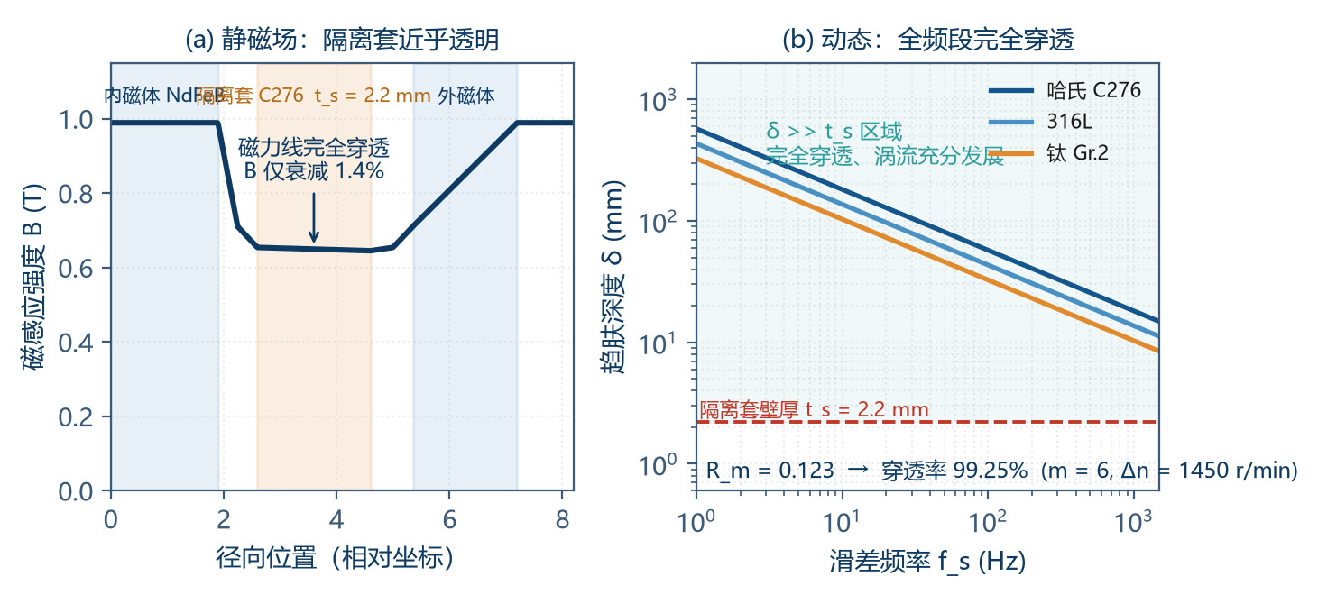
The core characteristic of the non-magnetic containment can is relative permeability µ_r ≈ 1 (austenitic stainless steel 1.005 – 1.02, Hastelloy 1.000 – 1.005, titanium 1.000, PEEK / SiC / ceramic 1.000). This means it is almost "transparent" to static magnetic field — no magnetic shunt, no flux shielding, only lengthening the magnetic circuit by t_s.
Therefore, the static effect of the containment can on the magnetic circuit is fully captured in the effective air gap:
This "transparency" has a cost. For the worked example, without the containment can the effective air gap is only 1.0 mm; with a 2.2 mm can it increases to 3.2 mm, and the permeance coefficient drops sharply from 14/(1.0·1.30) = 10.8 to 14/(3.2·1.30) = 3.37, moving the magnet working point far from B_r. This is the fundamental reason why magnetic couplings must be larger in volume than same-power ordinary couplings.
| Can Thickness t_s (mm) | Effective Gap g_eff (mm) | Permeance Coefficient P_c | Working Point B_m (T) | Working-Point |H_m| (kA/m) | Anti-Demag Verdict |
|---|---|---|---|---|---|
| 0 (no can, reference) | 1.0 | 10.77 | 1.184 | 87 | Excellent (impractical) |
| 0.8 | 1.8 | 5.98 | 1.104 | 147 | Excellent |
| 1.4 | 2.4 | 4.49 | 1.057 | 187 | Good |
| 2.0 | 3.0 | 3.59 | 1.007 | 223 | Acceptable |
| 2.2 (worked example) | 3.2 | 3.37 | 0.989 | 234 | Acceptable (lower-limit zone) |
| 3.0 | 4.0 | 2.69 | 0.914 | 271 | Low; high risk |
| 4.0 | 5.0 | 2.15 | 0.833 | 308 | Not acceptable |
Table 2-1 Effect of can thickness on the magnetic circuit (l_m = 14 mm, k_L = 1.30, N42SH)
Table 2-1 gives a clear design red line: the effective air gap should not exceed 1/4 - 1/3 of the magnet thickness. If pressure-resistance forces a thicker containment can, the magnet thickness l_m must be increased in step to maintain P_c, otherwise anti-demagnetisation capability will fall off a cliff.
2.3 Skin Depth & Magnetic Reynolds Number — Quantitative Proof of Penetration
Section 2.2 discusses static magnetic field. When the inner and outer rotors have relative slip, eddy currents are generated in the containment can, and the eddy field reacts back on the original field, forming "magnetic shielding". Two dimensionless criteria judge the degree of penetration.
2.3.1 Criterion 1 — Skin Depth δ
where ρ_e is the can's resistivity, f_s the slip frequency, m the pole-pair number, Δn the slip speed. When δ >> t_s, the alternating field fully penetrates and eddy currents develop fully through the wall thickness.
| Can Material | Resistivity ρ_e (µΩ·cm) | Relative Permeability µ_r | Skin Depth δ (mm) | δ / t_s Ratio* | Penetration Verdict |
|---|---|---|---|---|---|
| Hastelloy C276 | 130 | 1.000 – 1.005 | 47.7 | 21.7 | Fully penetrated; eddy currents fully developed |
| 316L stainless | 74 | 1.005 – 1.020 | 36.0 | 16.4 | Fully penetrated |
| Titanium Gr.2 | 42 | 1.000 | 27.1 | 12.3 | Fully penetrated (highest eddy loss) |
| PEEK / CFRP / SiC | 10¹⁶ - 10²⁰ | 1.000 | > 10⁶ | — | Insulator; no eddy current |
Table 2-2 Skin depth of different materials (f_s = 145 Hz, m = 6, Δn = 1450 r/min)
* Calculated with t_s = 2.2 mm of the worked example.
Conclusion 1: across the full operating-frequency range of a magnetic pump (normal synchronous f_s ≈ 0, pull-out f_s up to -600 Hz), the skin depth is always more than an order of magnitude greater than the can thickness. Therefore the containment can is "transparent" magnetically — flux is not attenuated; but precisely because of full penetration, eddy currents develop through the whole wall thickness and dissipation is maximised. These two seemingly contradictory conclusions are in fact two sides of the same physical reality.
2.3.2 Criterion 2 — Magnetic Reynolds Number R_m
Skin depth measures "whether penetration is possible"; magnetic Reynolds number measures "how strong the eddy back-reaction is". Definition:
R_m is the ratio of "convection term / diffusion term", the magnetic-diffusion-equation equivalent of the hydrodynamic Reynolds number. R_m << 1 means the eddy field is much smaller than the original field, and shielding is negligible. The flux penetration rate can be estimated by:
Substituting the worked-example values (C276: σ = 7.69×10⁵ S/m; slip Δω = 151.8 rad/s; R = 0.040 m; τ_p = 0.0209 m):
Conclusion 2: even at the worst-case full-pull-out duty (s = 1), the flux penetration rate is still as high as 99.25 %, and the eddy shielding effect is less than 1 %. Two engineering implications: (1) even at pull-out, the magnetic coupling still transmits considerable asynchronous torque (measured at 0.5 – 0.8 × T_max), which is precisely why the slip power is so large — the energy-input channel has not been cut off; (2) attempts to "thicken the metal can to shield the magnetic field" are futile; the only effective path is to raise resistivity or switch to a non-metallic material.
2.4 The Two Faces of Eddy Current — Static Transparency vs Dynamic Dissipation
Combining §2.2 and §2.3, the magnetic-electrical behaviour of the containment can is summarised in a unified picture:
| Duty | Slip Frequency f_s | Flux Penetration | Eddy Strength | Loss Magnitude | Engineering Meaning |
|---|---|---|---|---|---|
| Normal synchronous run | ≈ 0 (only harmonic) | Complete | Very weak | 0.5 – 2 % of rated | High efficiency; negligible |
| Start / load fluctuation | 0 – 30 Hz | Complete | Weak | 2 – 8 % of rated | Acceptable briefly; limit start frequency |
| Pull-out | 50 – 600 Hz | Complete | Strong | Equal to slip power (up to several × rated) | Must cut power within 5 s |
| Locked rotor (inner rotor stuck) | = supply-frequency value | Complete | Strongest | Maximum | Most dangerous; needs dual protection |
Table 2-3 Magnetic-electrical behaviour of the containment can under different duties
One point worth clarifying: the eddy current in the containment can is not purely negative. At start, eddy provides additional asynchronous starting torque, allowing the magnetic pump to start "under load" rather than "must be unloaded"; under brief overload, the asynchronous torque can carry the load above T_max for a short time, avoiding immediate pull-out. This "asynchronous margin" is valuable, but its cost is heat and cannot be sustained.
2.5 Model Verification Methods
The engineering credibility of the analytical model above must be validated through three routes:
Finite-element verification (recommended): build a 2D/3D transient electro-magnetic–thermal coupled FE model, solve Maxwell's equations, and obtain the spatial distribution of air-gap flux density, eddy-current density and loss. The analytical model is used for rapid scheme optimisation; FEA is used for final confirmation. The deviation between the two is typically 8 – 15 %.
Static-torque test: install a torque sensor or lever-loading device at the magnetic-coupling output, slowly load to pull-out, and record the measured T_max. This is the most direct way to verify the T_max analytical formula.
Temperature-rise measurement: attach K-type thermocouples to the outer wall of the containment can (metal can) or use infrared thermometry (non-metallic can), deliberately induce pull-out, record the temperature-rise curve, and back-calculate the eddy distribution coefficient k_sh. This is the experimental origin of k_sh = 0.85 (metal) and 0.02 (ceramic) in Chapter 4.
3 Synchronous Torque Characteristics & Torque Lock
3.1 Torque–Torque-Angle Characteristic
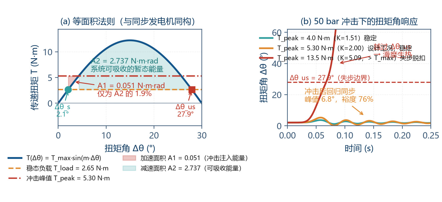
The torque of a synchronous magnetic coupling comes from the angular deviation Δθ (torque angle) between the inner- and outer-rotor pole axes. When Δθ = 0, the poles are fully aligned with no tangential force and torque is zero; as Δθ grows the tangential force grows, reaching its maximum at Δθ = 90°/m (electrical angle):
This relation is completely isomorphic to the power-angle characteristic of a synchronous generator, P = P_max·sin δ, which is the foundation for transplanting the Equal-Area Criterion below.
The maximum synchronous torque (pull-out torque) can be derived from the Maxwell stress tensor or the energy method:
where B_g is the fundamental air-gap flux-density amplitude (T), D the mean air-gap diameter (m), L the coupling axial length (m), η_c the magnetic-circuit coupling efficiency (0.45 – 0.70, including leakage and end effects), k_w the structural coefficient (0.85 – 0.95).
Key tip: T_max ∝ B_g², while B_g ∝ B_r ∝ (1 + α·ΔT). Therefore the temperature effect on torque is square-amplified — a 15.6 % B_r drop at 150 °C gives a 28.8 % torque drop. This is the quantitative root of thermal-runaway positive feedback and the reason why anti-demagnetisation design must leave enough margin.
Substituting the worked-example values (B_g = 0.490 T, D = 0.080 m, L = 0.045 m, η_c = 0.55, k_w = 0.90):
3.2 T_max Parameter Sensitivity
Understanding the weight of each parameter on T_max is the basis for optimisation:
| Parameter | Relation | T_max Change for +10 % | Optimisation Cost | Cost-Performance |
|---|---|---|---|---|
| Air-gap flux density B_g | T_max ∝ B_g² | +21.0 % | Thicker magnet or higher grade, cost ↑↑ | ★★★★★ |
| Coupling diameter D | T_max ∝ D² | +21.0 % | Volume ↑↑, can cost ↑↑, inertia ↑ | ★★★☆☆ |
| Coupling length L | T_max ∝ L | +10.0 % | Axial size ↑, can L/D worsens | ★★★★☆ |
| Effective gap g_eff | Via B_g; ≈ T_max ∝ g_eff⁻¹·⁶ | −13.7 % | Tighter gap needs higher machining accuracy | ★★★★★ |
| Pole pairs m | Weak (via η_c, k_w) | ±3 % | Affects frequency & eddy current | ★★☆☆☆ |
| Magnet thickness l_m | Via B_g saturation | +4 % - +7 % | Volume & cost ↑ | ★★★☆☆ |
Table 3-1 T_max parameter sensitivity (each parameter +10 %, worked example as baseline)
The most important conclusion in the table: reducing the effective air gap is the highest cost-performance optimisation — it even outperforms increasing the diameter. This points directly at the "containment-can minimisation" main line in Chapter 6.
In addition, raising B_g is effective but constrained: (1) high-grade magnets (N52 / N54) have lower H_cJ, so anti-demag degrades; (2) higher B_g strengthens the working-point field, raising demag risk. Pursuing high B_g and pursuing anti-demag is a contradiction; trade-off by working temperature tier is necessary — this is the theme of Chapter 5.
3.3 Three-Tier Definition of Torque Lock
This paper proposes the concept of "torque lock" (Anti-Decoupling) as the composite capability of a magnetic-coupling system to maintain synchronism across the full duty envelope. It is not a single index but three tiers of AND logic:
| Level | Physical Meaning | Quantitative Criterion | Worked-Example Check |
|---|---|---|---|
| L1 Static Lock | Margin of T_max over load torque at rated duty | SF_static = T_max(T) / T_rated ≥ 1.5 (≥ 1.3 at max T) | RT: 10.7/2.25 = 4.76; 150 °C: 7.62/2.25 = 3.39 → Pass |
| L2 Dynamic Lock | Torque angle does not cross unstable equilibrium under transient shock (Equal-Area) | K_imp = T_peak / T_max(T_max_temp) ≤ 0.65 | 4.50 / 7.62 = 0.591 → Pass |
| L3 Thermal Lock | Time from pull-out to demag T must exceed protection-action time | t_window = ΔT_demag / (dT/dt) ≥ 3 × t_protect | Metal can 20.8 s / 3 s = 6.9; Ceramic 333 s / 3 s = 111 → Pass |
Table 3-2 Three-tier torque-lock criteria
All three tiers must be met simultaneously; failure of any one tier means the design is unqualified. In engineering practice L1 is usually the easiest to meet (natural design margin), while L2 and L3 are the most easily ignored — yet field failures happen precisely in these two tiers.
3.4 Pull-out Dynamics — Isomorphism with Synchronous Generators
Consider the relative motion of the inner and outer rotors. Let the rotor angles be θ_i, θ_o and the torque angle Δθ = θ_o − θ_i. Writing the rotation equation for both rotors and eliminating the common term gives:
This is mathematically completely isomorphic to the swing equation of a synchronous generator: J·δ″ + D·δ′ + P_max·sin δ = P_mech. Therefore the mature Equal-Area Criterion from power-system transient stability analysis can be transplanted directly:
Accelerating area A₁ = ∫[T_peak − T_max·sin(m·Δθ)] dΔθ — kinetic energy gained by the rotor during the shock;
Decelerating area A₂ = ∫[T_max·sin(m·Δθ) − T_load] dΔθ — kinetic energy the system can absorb after the shock;
Stability criterion: A₁ ≤ A₂.
For a typical shock waveform (rectangular pulse, amplitude T_peak, duration t_p), the critical condition can be obtained analytically. The more practical engineering form is the critical iMPact coefficient:
3.5 Torque Spectrum under 50-bar Pressure Shock
The torque of a 50-bar system is not a single value but a spectrum stacked from four components. Design must identify all four:
| Torque Component | Formula | Value (N·m) | Share | When It Occurs | Avoidable? |
|---|---|---|---|---|---|
| ① Steady Δp torque | T_Δp = Δp·q/(2π·η_m) = 5.0×10⁶×2.4×10⁻⁶/(2π×0.85) | 2.25 | 50 % | Continuous | No (process necessity) |
| ② Mechanical friction torque | Bearing + gear mesh + face friction | 0.35 – 0.55 | 8 – 12 % | Continuous | Yes (bearing selection, clearance) |
| ③ Inertial acceleration torque | T_J = J·dω/dt (start / speed change) | 0.3 – 1.2 | 7 – 27 % | Start-stop, speed change | Yes (VFD soft start) |
| ④ Pressure-shock torque | Water hammer, fast valve, compressibility | Rated × 1.5 – 3.0 | Instantaneous overlay | Valve action, pump start-stop | Yes (slow-open valve, accumulator) |
| Combined rated torque | ① + ② | 2.60 – 2.80 | 100 % | — | — |
| Design peak torque T_peak | (① + ②) × iMPact coefficient 2.0 | 4.50 – 5.60 | — | — | — |
Table 3-3 Load-torque spectrum of a 50-bar magnetic gear pump (q = 2.4 mL/rev, n = 1450 r/min)
This paper takes T_peak = 4.50 N·m (iMPact coefficient 2.0) as the design input. Note: the iMPact coefficient of 2.0 applies to systems with slow-open valves + VFD soft start; if fast-open valves, long-pipe water hammer or high-viscosity media cold start exist, the iMPact coefficient should be 2.5 – 3.0, and T_peak will reach 6.5 – 8.4 N·m — the L2 criterion (≤ 0.65) will no longer hold. This shows that shock protection is not an "option" but a precondition for L2 lock to hold.
One easily overlooked duty is dry running. Magnetic pumps rely on the pumped medium to lubricate the internal sliding bearings (typically SiC or graphite). Once inlet flow is lost:
sliding bearing shifts from fluid lubrication to dry friction; friction coefficient jumps from 0.001 – 0.005 to 0.15 – 0.35, friction torque surges 30 – 80×;
medium cooling is also lost, deteriorating the can's heat dissipation;
5 – 15 seconds of dry running can push the temperature above 300 °C — the fastest demagnetisation path.
Therefore dry-running protection (differential-pressure switch / power monitor / temperature monitor, three-out-of-two) is mandatory for magnetic pumps, and should be an interlock-stop condition in semiconductor and chemical industries.
3.6 Re-Synchronisation Capability — The Self-Rescue Window after Pull-out
Pull-out does not inevitably cause demagnetisation. If the system can re-synchronise before the magnet temperature reaches the demagnetisation threshold, the damage is reversible. After pull-out the inner rotor enters asynchronous operation; its asynchronous torque is given by the Kloss formula:
where s_c is the critical slip (typical 0.25 – 0.45 for magnetic couplings). Re-synchronisation requires:
load torque drops below T_max(T) (e.g. via depressurisation, throttle outlet);
asynchronous torque is enough to accelerate the inner rotor back to synchronous speed, i.e. T_async > T_load;
this process takes less than the protection time window t_window.
In the worked example, after pull-out s = 1, s_c = 0.35: T_async = 6.67 N·m, still higher than rated load 2.25 N·m. This looks optimistic, but the cost is 1 012 W of slip power all converted to heat — therefore re-synchronisation capability only buys time, it cannot replace power-off protection. The correct engineering practice: after detecting pull-out, first unload (derate / depressurise) to attempt re-sync; if not restored within 3 seconds, cut power immediately.
4 Slip-Induced Heat — Thermal Runaway Mechanism after Pull-out
4.1 Slip Power — A Result Guaranteed by Energy Conservation
After pull-out, the outer rotor continues at synchronous speed ω_sync while the inner rotor decelerates to ω_i under load; the slip is Δω = ω_sync − ω_i. The magnetic coupling degrades to asynchronous (eddy) coupling, still transmitting torque T_async. By energy conservation, the difference between mechanical power input and output must all be converted to heat:
The importance of this formula is: it depends on no eddy-distribution detail, and is a direct consequence of the first law of thermodynamics. By contrast, directly using an eddy-loss formula such as the thin-plate formula P = π²B²f²t²V/(6ρ) brings order-of-magnitude errors — because the eddy loop characteristic length of the containment can is the "pole pitch" (-21 mm) rather than the "wall thickness" (-2 mm), and the geometric premise of the thin-plate formula does not hold.
Substituting the worked example:
| Step | Formula | Result |
|---|---|---|
| Synchronous angular velocity ω_sync | ω = 2πn/60 | 151.8 rad/s |
| Slip frequency f_s | f_s = m·Δn/60 = 6×1450/60 | 145 Hz |
| Critical slip s_c | By magnetic-circuit design | 0.35 |
| Full slip s | s = Δω/ω_sync = 1.0 (inner rotor locked) | 1.00 |
| Asynchronous torque T_async | 2·T_max·(s/s_c)/[1+(s/s_c)²] = 2×10.7×2.857/(1+8.163) | 6.67 N·m (= 0.62·T_max) |
| Slip power P_slip | P = T_async·Δω = 6.67×151.8 | 1 012 W |
| CoMParison: rated output power | P_out = T_load·ω = 2.25×151.8 | 342 W |
| Power amplification factor | P_slip / P_out | 2.96× |
Table 4-1 Slip-power calculation at pull-out (T_max = 10.7 N·m, m = 6, n = 1450 r/min)
A 342 W pump must dissipate 1 012 W of thermal power in the containment can and adjacent components after pull-out — almost three times rated output. This is the root cause of rapid magnetic-pump burn-out after pull-out.
4.2 Spatial Distribution of Heat
The slip power is distributed among three components according to the electromagnetic-field distribution: containment can (eddy), inner-magnet magnets (eddy), back iron & core (eddy + hysteresis). The distribution coefficients depend on material resistivity and whether segmental insulation is adopted:
| Component | Metal-Can Scenario (C276 / 316L / Ti) | Non-Metallic-Can Scenario (SiC / PEEK / CFRP) | Loss-Reduction Measure |
|---|---|---|---|
| Containment can | k_sh = 0.75 – 0.92 | k_sh = 0.01 – 0.03 | Raise resistivity; switch to non-metal |
| Inner-magnet magnets | k_m = 0.05 – 0.15 | k_m = 0.15 – 0.35 | Axial magnet segmentation + insulation between segments |
| Back iron / core / others | k_y = 0.03 – 0.15 | k_y = 0.10 – 0.30 | Silicon-steel lamination, slotting |
| Total | 1.00 | 1.00 | — |
| Can heat (worked example) | 1 012 × 0.85 = 861 W | 1 012 × 0.02 = 20 W | 43× difference |
Table 4-2 Slip-power distribution coefficients k (typical)
Note a counter-intuitive phenomenon: the metal containment can actually "protects" the magnet during pull-out — it absorbs 85 % of the heat, slowing the magnet's temperature rise; the price is that the can itself overheats, may burn out or deform, leading to medium leakage (can rupture = seal failure, the worst magnetic-pump accident mode).
Therefore the two scenarios have different risk profiles:
Metal-can: the can fails first (fast, -20 s); failure mode is "leakage", but with an obvious T-rise warning signal;
Non-metal-can: the can is safe; heat transfers to the magnet; failure mode is "demag", T-rise slow but warning signal weak (magnet T is hard to measure directly).
Engineering optimum: non-metallic can + magnet segmental insulation + inner-rotor online temperature monitoring, avoiding both failure modes simultaneously.
4.3 Temperature-Rise Dynamics
The temperature rise of the containment can (or magnet) can be described by a first-order lumped thermal model:
At the initial stage of pull-out (t << τ_th), heat dissipation is negligible and the temperature rise is approximately linear:
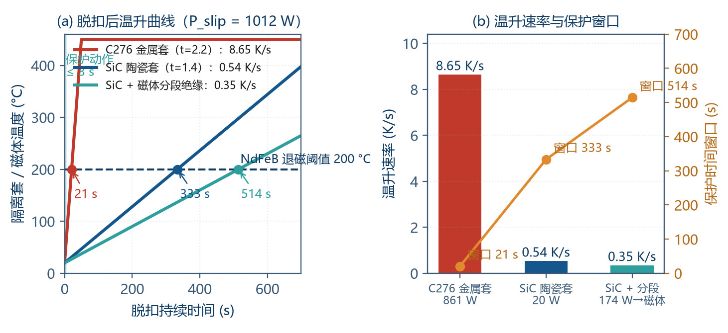
| Scenario | Component | Mass m (kg) | Specific Heat c (J/(kg·K)) | Allocated Power (W) | Heating Rate dT/dt (K/s) | Time to Reach 200 °C |
|---|---|---|---|---|---|---|
| C276 metal can (t = 2.2 mm) | Can | 0.221 | 450 | 861 | 8.65 | 20.8 s |
| C276 metal can (t = 2.2 mm) | Inner-magnet | 1.084 | 460 | 152 | 0.30 | 600 s |
| SiC ceramic can (t = 1.4 mm) | Can | 0.049 | 750 | 20 | 0.54 | 333 s |
| SiC ceramic can (t = 1.4 mm) | Inner-magnet | 1.084 | 460 | 355 | 0.71 | 253 s |
| SiC can + segmented magnet | Inner-magnet | 1.084 | 460 | 152 | 0.30 | 600 s |
Table 4-3 Heating rate coMParison after pull-out (worked example, P_slip = 1 012 W)
The data reveals the core contradiction and time window of protection design:
The metal-can protection window is only -21 seconds. Considering sensor response, PLC scan cycle and contactor opening time (combined 0.5 – 2 s), the time left for manual intervention is essentially zero; automatic interlocks must be relied on.
The ceramic-can scenario extends the window to 5.6 minutes, providing substantial space for diagnosis and intervention — reliability improves by an order of magnitude.
However, the final bottleneck is the magnet itself (253 – 600 s). If the pull-out state persists more than 10 minutes, demag still occurs. "Extended window" does not mean "immunity".
4.4 Quantitative Positive Feedback of Thermal Runaway
Coupling the temperature effect on magnetic performance with the slip power, the gain of thermal runaway can be quantified. After temperature rise ΔT:
Taking α = −0.12 %/K, the temperature coefficient of T_max is 2α = −0.24 %/K, i.e. each 100 K of temperature rise reduces T_max by -21 %.
Runaway criterion: if the T_max decay rate caused by temperature rise exceeds the load-torque decay rate (or the system's design-margin absorption capability), the system enters irreversible runaway. A simplified engineering criterion is:
In the worked metal-can example: dT/dt = 8.65 K/s, |dT_max/dT| = 0.24 %/K, product = 2.08 %/s, exceeding the 0.3 %/s threshold by 6.9× — explaining why metal-can magnetic pumps are almost unable to self-rescue after pull-out.
4.5 Dry Running — The Most Dangerous Duty
Of all pull-out triggers, dry running is the most harmful because it simultaneously destroys "lubrication" and "cooling":
| Item | Normal Duty | Dry-Running Duty | Worsening Factor |
|---|---|---|---|
| Internal bearing lubrication | Hydrodynamic, µ_f = 0.001 – 0.005 | Dry friction, µ_f = 0.15 – 0.35 | 30 – 80× |
| Bearing friction torque | 0.05 – 0.10 N·m | 1.5 – 4.0 N·m | 15 – 40× |
| Can heat dissipation | Medium forced conv., α = 500 – 3 000 W/(m²·K) | Gas natural conv., α = 5 – 25 W/(m²·K) | Dissipation falls to 1/100 |
| Can thermal time constant τ_th | 3 – 10 s | 150 – 400 s | Dissipation basically fails |
| Time to reach 300 °C | Never (medium cooling) | 5 – 15 s | — |
| Typical trigger | — | Inlet starvation, filter clog, cavitation, valve mis-close, low level | — |
Table 4-4 Normal vs dry-running coMParison
Minimum dry-running protection configuration (three-out-of-two interlock):
Inlet pressure / level switch: alarms and interlocks when inlet pressure falls below the threshold;
Motor-power monitor: power anomalously drops in dry-running (because medium density falls);
Pump-body temperature monitor: install temperature switches on the can outer wall or pump cover.
For semiconductor, pharmaceutical and other continuous-production industries, a 2oo3 redundant configuration is recommended, avoiding single-point misoperation causing unplanned shutdown while avoiding single-point failure causing protection loss.
5 Extreme-Temperature Anti-Demagnetisation Design
5.1 NdFeB Demagnetisation Curve & Knee-Point Mechanism
The second-quadrant demagnetisation curve (B-H curve) of NdFeB is the starting point of anti-demagnetisation design. Its typical shape: approximately horizontal at low demagnetising field (slope = µ_0·µ_rc), then sharply drops at some point — this point is called the knee point, with field strength H_k.
The physical meaning of the knee point: when the external demagnetising field exceeds H_k, part of the magnetic moments of internal grains undergo irreversible flip (reverse-domain nucleation and growth). Once this happens, even if the external field is removed, the magnetic moments do not automatically recover — this is irreversible demagnetisation (permanent magnetic-performance loss).
| Grade | B_r (T) | H_cB (kA/m) | H_cJ (kA/m) | (BH)_max (kJ/m³) | α(B_r) (%/K) | β(H_cJ) (%/K) | Nominal Max T |
|---|---|---|---|---|---|---|---|
| N42 | 1.30 | ≥ 955 | ≥ 955 | 318 – 342 | −0.12 | −0.65 | 80 °C |
| N45 | 1.35 | ≥ 955 | ≥ 955 | 342 – 366 | −0.12 | −0.65 | 80 °C |
| N48 | 1.38 | ≥ 955 | ≥ 955 | 358 – 382 | −0.12 | −0.65 | 80 °C |
| N42M | 1.30 | ≥ 995 | ≥ 1114 | 318 – 342 | −0.12 | −0.60 | 100 °C |
| N42H | 1.30 | ≥ 995 | ≥ 1273 | 318 – 342 | −0.12 | −0.58 | 120 °C |
| N42SH | 1.30 | ≥ 987 | ≥ 1592 | 318 – 342 | −0.12 | −0.55 | 150 °C |
| N40UH | 1.26 | ≥ 939 | ≥ 1990 | 302 – 326 | −0.12 | −0.50 | 180 °C |
| N38EH | 1.24 | ≥ 915 | ≥ 2387 | 287 – 310 | −0.12 | −0.47 | 200 °C |
| N35AH | 1.18 | ≥ 875 | ≥ 2785 | 263 – 287 | −0.12 | −0.45 | 230 °C |
Table 5-1 Common sintered NdFeB grades performance (20 °C) and temperature coefficient
Data are industry-typical; specific manufacturers and batches differ. Please refer to the supplier's formal specification for selection. H_cJ is the minimum-value guarantee; the actual measured typical value is usually 5 – 15 % higher than the tabulated number.
Reading the table: raising the temperature grade is at the cost of B_r for H_cJ. From N42 to N38EH, H_cJ increases 150 % (955 → 2 387 kA/m) while B_r only drops 4.6 % (1.30 → 1.24 T). Considering T_max ∝ B_r², a 4.6 % B_r drop only reduces torque by 9 %, while anti-demagnetisation capability is greatly improved — this is the first principle of extreme-temperature design: sacrifice a small amount of magnetic energy product to ensure sufficient intrinsic coercivity.
5.2 Temperature Coefficient — Different Fates of B_r and H_cJ
Temperature affects the two key parameters of NdFeB very asymmetrically:
The absolute value of β is 4 – 6× that of α. This means the decay of anti-demag capability with temperature is much faster than the decay of magnetic-flux density. Example: temperature from 20 °C to 150 °C (ΔT = 130 K):
| Grade | B_r Retention | H_cJ Retention | H_k Retention* (H_k ≈ 0.9·H_cJ) | T_max Retention (∝ B_r²) | Verdict |
|---|---|---|---|---|---|
| N42 | 84.4 % | 15.5 % | 15.5 % | 71.2 % | H_cJ collapses — inevitable demag |
| N42H | 84.4 % | 24.6 % | 24.6 % | 71.2 % | H_cJ insufficient; high risk |
| N42SH | 84.4 % | 28.5 % | 28.5 % | 71.2 % | Usable (used in this paper) |
| N40UH | 84.4 % | 35.0 % | 35.0 % | 71.2 % | Good |
| N38EH | 84.4 % | 38.9 % | 38.9 % | 71.2 % | Excellent (200 °C class) |
Table 5-2 Magnetic-performance retention at 150 °C of each grade
* Assumes H_k has the same temperature coefficient as H_cJ (engineering approximation; measured H_k decay is slightly faster).
The most striking number in Table 5-2: N42 at 150 °C retains only 15.5 % H_cJ (148 kA/m). At this point any normal load fluctuation can push the working point beyond the knee point. This is why ordinary grades must never be used in high-temperature magnetic pumps.
Another important observation: the T_max retention rate is independent of grade (always 71.2 %), because T_max depends only on B_r, and all grades share the same B_r temperature coefficient. Grade choice affects "whether it can be used", not "how strong it is when used".
5.3 High-Temperature Side — Grade System & Grain-Boundary Diffusion
5.3.1 Grade Selection Rules
| Medium / Magnet Max Temperature | Recommended Grade | H_cJ (20 °C) Requirement | Note |
|---|---|---|---|
| ≤ 80 °C | N42 / N45 / N48 | ≥ 955 kA/m | RT duty; prioritise magnetic energy product |
| 80 – 120 °C | N42M / N42H | ≥ 1114 / 1273 kA/m | Mid-T; balance cost |
| 120 – 150 °C | N42SH | ≥ 1592 kA/m | Mainstream choice for hot oil, high-T reactors |
| 150 – 180 °C | N40UH | ≥ 1990 kA/m | Recommend combined with GBD |
| 180 – 200 °C | N38EH | ≥ 2387 kA/m | Recommend combined with GBD |
| 200 – 230 °C | N35AH | ≥ 2785 kA/m | NdFeB limit; low cost-performance |
| > 230 °C | Sm₂Co₁₇ | — | Must switch to Sm-Co (see §5.5) |
Table 5-3 NdFeB grade selection rule by working temperature (P_c ≥ 3.3, zero-irreversible-demag criterion)
5.3.2 Grain Boundary Diffusion (GBD) — The Highest Cost-Performance Anti-Demag Measure
The traditional method to raise H_cJ is to add heavy rare-earth Dy/Tb during melting. But Dy/Tb also reduces B_r (each 1 wt% Dy reduces B_r by -0.015 T and raises H_cJ by -200 kA/m), and heavy rare earths are expensive and resource-constrained.
Grain Boundary Diffusion (GBD) solves this contradiction: Dy/Tb is applied to the magnet surface by vapour, sputtering or coating, then thermally treated so it diffuses selectively along the grain boundary, forming a high-anisotropy-field "core–shell" structure on the outer layer of the main-phase grain, while the inside of the grain retains high-B_r pure Nd₂Fe₁₄B.
| CoMParison Item | Traditional Bulk Addition (Smelt-Dy) | GBD | Winner |
|---|---|---|---|
| H_cJ improvement | +30 – 60 % (equal Dy) | +30 – 60 % (equal Dy) | CoMParable |
| B_r loss | −0.010 – 0.020 T | −0.002 – 0.005 T | GBD significantly wins |
| (BH)_max loss | −5 – 12 % | −1 – 3 % | GBD significantly wins |
| Heavy-rare-earth usage | 2 – 6 wt% | 0.4 – 1.2 wt% | GBD uses only 1/5 |
| Cost increment | +40 – 80 % | +15 – 30 % | GBD wins |
| Thickness-limit applicability | None | < 8 – 10 mm (diffusion-depth limit) | Bulk wins |
| High-T demag loss (150 °C, P_c = 2) | −8 – 15 % | −2 – 5 % | GBD significantly wins |
Table 5-4 Grain-boundary diffusion vs traditional bulk Dy addition
Conclusion: for magnets with thickness ≤ 8 mm, GBD is the preferred anti-demag technique; for thicker magnets (e.g. worked-example l_m = 14 mm), use a "low-Dy bulk addition + GBD" combined scheme, or locally strengthen the demag-prone edges (magnet pole ends).
Two supporting technologies:
Magnet segmentation with insulation: divide the monolithic magnet axially into 4 – 12 segments, with insulating adhesive (epoxy + glass-fibre cloth) between segments; this cuts the eddy loop, reducing magnet eddy loss k_m from 0.15 – 0.35 to 0.03 – 0.08 and reducing magnet self-heating during pull-out by more than 70 %.
Grain refinement & grain-boundary optimisation: by controlling the sintering process to refine the grain (< 5 µm) and optimising the grain-boundary phase distribution, H_cJ can be raised by 10 – 20 % without adding heavy rare earth.
5.4 Cryogenic Side — The Illusion of B_r Rise & Spin-Reorientation Trap
The cryogenic end is often mistakenly considered "safer" because NdFeB B_r rises significantly at low temperature. Table 5-5 gives typical changes:
| Temperature | B_r Change | H_cJ Change | Magnetic-Performance Verdict | Main Risk |
|---|---|---|---|---|
| 0 °C | +2.4 % | +14 % | Better than RT | No significant risk |
| −40 °C | +7.2 % | +43 % | Optimal performance zone | CTE mismatch, adhesive embrittlement |
| −80 °C | +12.0 % | +71 % | Excellent performance | Structural stress, magnet cracking |
| −138 °C | +19.0 % | +112 % | Enters spin-reorientation zone | Magnetocrystalline anisotropy sudden change |
| −196 °C (LN₂) | +26.0 % | +154 % | Strongest apparent performance | Serious structural risk + unstable behaviour |
| −253 °C (LH₂) | — | — | Not recommended | Switch to Sm-Co or other systems |
Table 5-5 NdFeB performance change at low temperature (20 °C reference)
Table 5-5 reveals two cryogenic traps:
5.4.1 Trap 1 — Spin Reorientation
The easy-magnetisation direction of Nd₂Fe₁₄B changes at -135 K (−138 °C): the magnetic moment tilts away from the c-axis, forming an "easy cone" structure. This causes the magnetocrystalline anisotropy field to drop, observed as anomalous kinks in the temperature dependence of magnetic performance, hysteresis-loop distortion, and increased sensitivity to demagnetising fields.
Engineering meaning: when the magnet working temperature may fall below −130 °C, the room-temperature demagnetisation curve cannot be extrapolated; suppliers' cryogenic measured data must be requested, or switch to Sm₂Co₁₇. For LNG (−162 °C) transport and liquid-nitrogen pre-cooling, this point is especially important.
5.4.2 Trap 2 — Anisotropic Thermal Expansion
The thermal expansion of sintered NdFeB is anisotropic:
Stainless steel (16 × 10⁻⁶/K) and aluminium alloy (23 × 10⁻⁶/K) differ greatly. From +20 °C to −196 °C (ΔT = −216 K):
Difference 0.195 %. For a 40 mm fit size, this is 78 µm of relative displacement difference. With rigid bonding (high-modulus epoxy, fracture elongation < 1 %), the adhesive layer will crack under huge shear stress.
Cryogenic-magnet-assembly engineering countermeasures:
use low-modulus, high-elongation flexible adhesives (modified epoxy, polyurethane; fracture elongation > 30 %, T_g at least 20 K below the lowest working temperature);
add carbon-fibre (CFRP) banding ring as mechanical redundancy — even if the adhesive fails, the magnet position is maintained;
use "clearance fit + elastic element" mechanical fixing (e.g. wave-spring preload), avoiding interference fits;
CTE of all structural parts (magnet, can, back-iron, shaft) should be matched as much as possible, with differences controlled within 8 × 10⁻⁶/K.
5.5 Sm₂Co₁₇ vs NdFeB — Decision Rules
When the temperature exceeds the NdFeB capability boundary (> 230 °C or < −130 °C), samarium-cobalt (Sm-Co) is the only viable rare-earth permanent-magnet solution.
| Item | Sintered NdFeB (N42SH) | Sintered Sm₂Co₁₇ | Verdict |
|---|---|---|---|
| B_r (20 °C) | 1.30 T | 1.05 – 1.15 T | NdFeB wins (+13 – 24 %) |
| (BH)_max | 318 – 342 kJ/m³ | 200 – 260 kJ/m³ | NdFeB wins (+30 – 60 %) |
| H_cJ (20 °C) | 1 592 kA/m | 1 590 – 2 390 kA/m | CoMParable, Sm-Co slightly better |
| α(B_r) tempco | −0.12 %/K | −0.035 %/K | Sm-Co wins (only 1/3.4) |
| β(H_cJ) tempco | −0.55 %/K | −0.20 – −0.30 %/K | Sm-Co wins |
| Curie temperature T_c | 310 – 340 °C | 800 – 850 °C | Sm-Co wins significantly |
| Maximum working temperature | 150 °C (SH) / 230 °C (AH) | 300 – 350 °C | Sm-Co wins significantly |
| Cryogenic applicability | Limited by spin reorientation (−138 °C) | No spin reorientation, down to −269 °C | Sm-Co wins significantly |
| Oxidation / corrosion resistance | Poor; must be coated | Good; can be used bare (slight oxidation) | Sm-Co wins |
| Mechanical strength | Fair (flexural 250 – 350 MPa) | Brittle (flexural 100 – 150 MPa) | NdFeB wins |
| Machinability | Can be ground, wire-cut | Very brittle, only grinding; chipping-prone | NdFeB wins |
| Raw-material cost | Medium (Nd / Pr price dependent) | High (Sm & Co, 2 – 4× price) | NdFeB wins |
| Thermal-cycling stability | Large irreversible loss | Very small (< 1 % @ 300 °C ageing) | Sm-Co wins |
Table 5-6 Comprehensive coMParison of NdFeB vs Sm₂Co₁₇
The decision rules can be summarised in three:
Rule 1 (hard temperature boundary): T > 230 °C or T < −130 °C — must use Sm₂Co₁₇, no alternative.
Rule 2 (soft temperature boundary): 150 < T ≤ 230 °C or −130 ≤ T < −60 °C — make a technical-economic coMParison. If space is constrained and high power-density is required, choose NdFeB (AH/EH + GBD); if long-term stability and maintenance-free are required, choose Sm-Co.
Rule 3 (conventional range): −60 °C - +150 °C — NdFeB is the only reasonable choice (overwhelming cost and magnetic-energy-product advantage).
Note: Sm-Co's lower B_r means achieving the same T_max requires 20 – 35 % more coupling volume (T_max ∝ B_r²), which can become a decisive constraint in space-limited duties. Therefore in the mid-to-high temperature range, "NdFeB + GBD + enhanced cooling" is often chosen rather than directly switching to Sm-Co.
5.6 Anti-Demag Magnetic-Circuit Rule — The Minimum P_c Method
Integrating the mechanisms above, a complete anti-demagnetisation check procedure can be built, centred on the minimum permeance-coefficient method:
Step 1: determine the knee-point field strength of the magnet at the maximum working temperature T_max:
Step 2: determine the working-point field strength:
Step 3: apply the safety-margin criterion (this paper recommends 30 % margin, corresponding to zero irreversible demag):
Step 4: solve for the required minimum permeance coefficient P_c,min, then determine the magnet thickness and air gap:
For engineering use, Table 5-7 gives the minimum P_c required for each grade at each temperature (criterion: |H_m| ≤ 0.7·H_k, µ_rc = 1.06):
| Grade | 20 °C | 80 °C | 100 °C | 120 °C | 150 °C | 180 °C | 200 °C |
|---|---|---|---|---|---|---|---|
| N42 | 1.35 | 2.05 | 2.68 | 4.12 | 9.86 | Fail | Fail |
| N42H | 1.02 | 1.42 | 1.71 | 2.28 | 4.05 | 12.4 | Fail |
| N42SH | 0.82 | 1.10 | 1.28 | 1.60 | 2.47 | 5.02 | 13.7 |
| N40UH | 0.66 | 0.87 | 1.00 | 1.21 | 1.75 | 2.98 | 5.71 |
| N38EH | 0.55 | 0.72 | 0.82 | 0.98 | 1.37 | 2.16 | 3.63 |
| N35AH | 0.47 | 0.61 | 0.69 | 0.82 | 1.12 | 1.68 | 2.66 |
| Worked example: N42SH @ 150 °C, actual P_c = 3.37 ≥ 2.47 → 36 % margin → Pass | |||||||
Table 5-7 Minimum required permeance coefficient P_c,min per grade
Table 5-7 is one of the most practically useful tools in this paper. Usage: select the row by working temperature, read P_c,min, then by P_c = (l_m/g_eff)·(A_g/A_m)/k_L back-calculate magnet thickness or maximum allowed air gap.
Reading points:
The higher the temperature, the more non-linear the required P_c climbs (because H_cJ decays fast). N42 at 150 °C needs P_c ≥ 9.86, which cannot be realised in the large air-gap structure of a magnetic coupling — this is why N42 must never be used at 150 °C.
N42SH at 150 °C only needs P_c ≥ 2.47, and the actual design easily reaches 3.0 – 4.0, so SH is the mainstream choice at the 150 °C level.
N38EH at 200 °C only needs P_c ≥ 3.63, still achievable, so EH is a viable solution at the 200 °C level.
5.7 Magnet Fixing, Coating & Protection
Beyond the electrical design of the magnetic circuit, mechanical and chemical protection also determine service life:
| Protection Element | Technical Measure | Applicable Conditions | Key Parameters |
|---|---|---|---|
| Surface coating | Ni-Cu-Ni electroplating (standard) | General industrial environment, < 120 °C | Thickness 15 – 25 µm, salt spray ≥ 96 h |
| Surface coating | Epoxy e-coat / spray | Chemical corrosion environment | Thickness 20 – 40 µm, acid / alkali resistant |
| Surface coating | Parylene vapour deposition | Semiconductor high-purity, pinhole-sensitive | Thickness 5 – 15 µm, pinhole-free |
| Surface coating | Al ion-plating / PVD | High temperature (> 150 °C), no H-embrittlement | Thickness 8 – 15 µm |
| Mechanical fixing | High-strength anaerobic adhesive + epoxy | Routine | Shear strength ≥ 20 MPa |
| Mechanical fixing | CFRP banding ring | High speed, thermal cycling, redundancy required | Banding pre-stress 30 – 80 MPa |
| Mechanical fixing | Stainless / Ti can + interference | Strong corrosion, high speed | Interference 0.02 – 0.06 mm |
| Magnet segmentation | Axial 4 – 12 segments + insulating adhesive | All mid-to-high power magnetic pumps | Inter-segment insulation > 10 MΩ |
| H-embrittlement prevention | Avoid hydrogen-evolving plating | All NdFeB (H-absorption pulverisation risk) | Prefer PVD |
Table 5-8 Magnet protection system
Special tip: NdFeB is extremely sensitive to hydrogen — after absorbing hydrogen it undergoes intergranular fracture (hydrogen decrepitation), causing the magnet to powderise. Therefore after electroplating (hydrogen-evolving process), strict de-hydrogen baking must be done (180 – 220 °C, 2 – 4 h), or use non-hydrogen-evolving PVD in critical applications.
6 Engineering Solution for 50-bar Pressure Shock
6.1 The Trilemma of the Containment Can
The containment can is the only component in the magnetic pump simultaneously subject to three constraints — strength, magnetism and electrical — and its design is a typical multi-objective conflict problem:
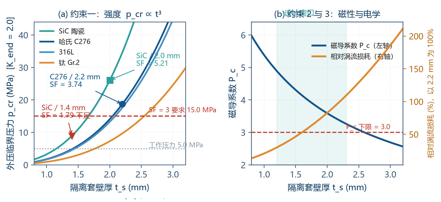
Strength dimension: external-pressure buckling requires wall thickness t_s as large as possible (p_cr ∝ t³);
Magnetic dimension: effective air gap requires t_s as small as possible (P_c ∝ 1/g_eff, T_max ∝ B_g²);
Electrical dimension: eddy loss requires resistivity as high as possible and thickness as small as possible (P_sh ∝ t²).
The intersection of the three is the design window. Constraint equations are built one by one below.
6.1.1 Constraint 1 — External-Pressure Buckling
The containment can has high-pressure medium inside and atmosphere outside — an external-pressure cylinder buckling problem. For long cylinders (large L/D, no intermediate support) the elastic critical pressure is given by Bresse's formula:
For short cylinders (end constraints or intermediate support rings) the critical pressure is significantly higher, with the end-constraint coefficient K_end correcting in engineering:
| Material | E (GPa) | ν | t_s (mm) | p_cr,long (MPa) | p_cr,design (MPa) | Safety Factor SF | Verdict |
|---|---|---|---|---|---|---|---|
| Hastelloy C276 | 205 | 0.30 | 1.5 | 2.97 | 5.94 | 1.19 | Not qualified |
| Hastelloy C276 | 205 | 0.30 | 2.0 | 7.04 | 14.08 | 2.82 | Critical |
| Hastelloy C276 | 205 | 0.30 | 2.2 | 9.35 | 18.69 | 3.74 | Pass (used in this paper) |
| Hastelloy C276 | 205 | 0.30 | 2.5 | 13.75 | 27.50 | 5.50 | Conservative |
| 316L | 193 | 0.30 | 2.2 | 8.80 | 17.60 | 3.52 | Pass but weaker corrosion resistance |
| Titanium Gr.2 | 103 | 0.34 | 2.2 | 4.83 | 9.66 | 1.93 | Not qualified (E too low) |
| SiC ceramic | 400 | 0.20 | 1.4 | 4.47 | 8.93 | 1.79 | Insufficient (brittle needs SF 4 – 6) |
| SiC ceramic | 400 | 0.20 | 2.0 | 13.02 | 26.05 | 5.21 | Pass, no eddy loss |
Table 6-1 External-pressure buckling check (D = 80 mm, p_op = 5.0 MPa, K_end = 2.0)
Table 6-1 hides an extremely important but often overlooked design lever: the critical pressure is inversely proportional to the diameter cubed (p_cr ∝ 1/D³). Reducing the coupling diameter from 80 mm to 60 mm, the critical pressure at the same wall thickness increases by (80/60)³ = 2.37×: a SiC containment can at D = 60 mm only needs 1.6 mm wall thickness to obtain 15.80 MPa critical pressure (SF = 6.32), while at D = 80 mm the same thickness gives only 6.67 MPa (SF = 2.67, not qualified). This means reducing diameter and increasing length is the single most powerful way to relieve the trilemma — it simultaneously allows thinner wall thickness, thereby shrinking the effective air gap, raising the permeance coefficient and reducing eddy loss; a rare "win-win-win" direction at the cost only of axial size. The rework scheme in Chapter 7 proceeds exactly along this direction.
An important finding in the table: although titanium alloy has excellent corrosion resistance, its elastic modulus is only 103 GPa (about half of C276), so the external-pressure stability at the same thickness is clearly insufficient, requiring thicker walls — which actually increases eddy loss. This corrects the common misunderstanding that "titanium can is the best".
Two additional corrections must be stacked:
Corrosion allowance: for corrosive media, add 0.2 – 0.5 mm corrosion allowance to the strength wall thickness;
Temperature derating: at high temperature E and allowable stress drop; at 200 °C, C276's E drops about 8 %, and the critical pressure drops in step.
6.1.2 Constraint 2 — Effective Air Gap & Permeance Coefficient
From Table 2-1 we know each 0.5 mm increase in t_s drops P_c by about 0.3 – 0.5. Within the design window, the two are strongly coupled. Therefore support rings (shortening the effective cylinder length to raise K_end) are the most economical means to crack the trilemma — it doesn't increase wall thickness but can raise the critical pressure by 1.5 – 4×.
6.1.3 Constraint 3 — Eddy-Current Loss
Eddy-current loss is inversely proportional to material resistivity and proportional to wall thickness squared. The resistivity ranking (high to low):
Note: titanium has the lowest resistivity and the highest eddy loss, stacking with the buckling disadvantage in §6.1.1. Titanium is the worst choice for a 50-bar magnetic-pump containment can (unless its chloride resistance is irreplaceable in a strong-chloride environment — in which case switch to Hastelloy C276 or ceramic).
6.2 Containment-Can Material Selection Matrix
| Material | Resistivity (µΩ·cm) | µ_r | E (GPa) | Applicable T | Eddy Loss | External-Pressure Stability | Corrosion Resistance | Cost |
|---|---|---|---|---|---|---|---|---|
| Hastelloy C276 | 130 | 1.00 | 205 | −200 - 500 °C | Medium | Excellent | Excellent | High |
| 316L | 74 | 1.01 | 193 | −200 - 400 °C | Medium-high | Good | Good | Low |
| Titanium Gr.2 | 42 | 1.00 | 103 | −250 - 300 °C | High | Poor | Excellent (Cl⁻ resistant) | Medium |
| PEEK (pure) | 10¹⁶ | 1.00 | 4 | −50 - 250 °C | None | Poor (E too low) | Excellent | Medium |
| PEEK-CF30 | 10²⁻⁴ | 1.00 | 13 | −50 - 250 °C | Very low | Poor | Excellent | Medium |
| SiC ceramic | 10¹¹ | 1.00 | 400 | −270 - 800 °C | None | Excellent | Excellent | High |
| Zirconia ZrO₂ | 10¹² | 1.00 | 210 | −270 - 600 °C | None | Excellent | Excellent | High |
| Al₂O₃ ceramic | 10¹⁴ | 1.00 | 350 | −270 - 700 °C | None | Excellent | Good (no HF / strong alkali) | Medium |
Table 6-2 Containment-can material selection matrix
Selection recommendations:
RT - 150 °C, 50 bar, general corrosion: Hastelloy C276 (t = 2.2 mm with support rings);
RT - 150 °C, 50 bar, strong corrosion or high-purity requirement: SiC ceramic (D = 80 mm requires t = 2.0 mm; if coupling diameter reduced to 60 mm, t = 1.6 mm suffices, with better magnetic performance);
Temperature > 200 °C: SiC or zirconia (metal can resistivity rises with temperature, eddy loss further worsens);
Pressure < 16 bar: consider PEEK-CF30 (clear cost advantage and no eddy);
HF-containing medium: forbidden Al₂O₃ and Si-containing materials; choose PEEK or Hastelloy C276.
6.3 Five Defence Lines — Anti Pull-out Protection
Based on the failure chain (Table 1-2), five defence lines are constructed. The line design follows "defence-in-depth": a single-point failure should not lead to catastrophic consequences.
| Line | Target Link | Technical Measures | Action Time | Failure Consequence (if this line fails) |
|---|---|---|---|---|
| First | Source suppression ① overload/shock | VFD soft start (accel time 8 – 20 s), slow-open valve, line accumulator, anti-siphon circuit | Continuous | VFD parameter + process valve selection |
| Second | Torque limit | VFD torque limit (set 0.6 – 0.7 T_max), mechanical shear pin (redundant) | < 100 ms | VFD + mechanical torque limiter |
| Third | Slip detection ② pull-out | Inner & outer rotor speed coMParison (dual encoder / Hall / eddy probe), pull-out if Δn > 5 % | 50 – 200 ms | PLC high-speed counter or dedicated module |
| Fourth | Unload & re-sync ② → ③ | Auto-derate to 30 – 50 %, throttle outlet control valve, try to pull back to sync | 1 – 3 s | VFD + control-valve linkage |
| Fifth | Fast power-off ③ slip heating | Main circuit contactor open + inlet emergency shut-off valve | < 3 s (total) | Safety-relay circuit (hard-wired, not via PLC) |
Table 6-3 Five defence lines against pull-out
Key design details among the five lines:
Third-line detection principle: the most reliable method is dual-speed coMParison (one speed sensor at each end of the outer rotor and the inner rotor). Since the inner rotor is inside the containment can and cannot host an encoder directly, the actual practice is to cut a non-magnetic window in the pump body and use a Hall sensor or eddy-current probe to sense the inner-rotor magnetic-pole frequency, coMParing it with the outer-rotor (motor encoder) frequency.
Fifth line must be hard-wired: PLC scan cycle, communication delay, and software failure can all cause protection failure. The safety-relay circuit must be independent of the control system, triggered directly by the dry-contact of the temperature switch or slip-detection relay.
Temperature-monitoring location: in the metal-can scenario, mount a PT100 on the outer wall axial midpoint of the containment can (response < 1 s); in the ceramic-can scenario, the can itself does not heat up, so monitor the pump-body medium outlet temperature and motor current for indirect judgement.
6.4 Recommended Control Strategy Parameters
| Parameter | Recommended Value | Rationale |
|---|---|---|
| VFD acceleration time | 10 – 20 s | Limit inertial torque T_J < 0.3·T_max |
| VFD deceleration time | 15 – 30 s | Prevent water hammer & reverse rotation |
| Torque-limit setpoint | 0.65 × T_max(T_max_temp) | Corresponding to L2 dynamic-lock criterion |
| Current-limit setpoint | 1.1 × rated current | Prevent motor overload |
| Slip pull-out criterion | Δn/n > 5 %, sustained > 200 ms | Avoid transient slip at start-up |
| Temperature alarm threshold | T_shell > 120 °C alarm | ≥ 60 K below demag T |
| Temperature stop threshold | T_shell > 160 °C stop | 40 K safety margin |
| Dry-running protection | Inlet P < 0.05 MPa or Power < 60 % rated | Dual-criterion OR |
| Start-frequency limit | ≤ 6 / hour | Limit cumulative eddy heat |
Table 6-4 Recommended 50-bar magnetic-pump control parameters
6.5 Design Verification Checklist
Summarising the full text, a 12-step design verification checklist is formed for design review:
| # | Check Item | Criterion | Reference |
|---|---|---|---|
| 1 | Load-torque spectrum | T_rated and T_peak have all four components identified | 3.5 |
| 2 | Effective air gap | g_eff ≤ l_m / 3.5 | 2.2 |
| 3 | Permeance coefficient | P_c ≥ 3.0 (RT) / ≥ 3.5 (high T) | 2.1 |
| 4 | Flux penetration | δ / t_s > 10 and R_m < 0.3 | 2.3 |
| 5 | Maximum synchronous torque | T_max(20 °C) by analytical formula, verified by FEA or measurement | 3.1 |
| 6 | L1 static lock | T_max(T_max_temp) / T_rated ≥ 1.3 | 3.3 |
| 7 | L2 dynamic lock | T_peak / T_max(T_max_temp) ≤ 0.65 | 3.3 / 3.4 |
| 8 | Containment-can external-pressure buckling | K_end · p_cr ≥ 3.0 · p_op (incl. corrosion allowance & T derating) | 6.1.1 |
| 9 | Eddy distribution & T-rise | dT/dt and protection time window quantified | 4.2 / 4.3 |
| 10 | L3 thermal lock | t_window ≥ 3 × t_protect | 3.3 |
| 11 | Grade & minimum P_c | From Table 5-7, P_c,actual ≥ P_c,min(T_max) | 5.6 |
| 12 | Protection system | All five defence lines in place, fifth line hard-wired | 6.3 |
Table 6-5 12-step magnetic-coupling design verification checklist
7 Design Worked Example — Complete Verification Procedure
7.1 Design Inputs
| Item | Symbol | Value | Unit |
|---|---|---|---|
| Pump displacement | q | 2.4 | mL/rev |
| Rated speed | n | 1450 | r/min |
| Design pressure difference (50 bar) | Δp | 5.0 | MPa |
| Mechanical efficiency | η_m | 0.85 | — |
| Medium maximum temperature | T_max | 150 | °C |
| IMPact coefficient | K_imp | 2.0 | — |
| Magnetic-coupling air-gap mean diameter | D | 80 | mm |
| Coupling axial length | L | 45 | mm |
| Magnet thickness | l_m | 14 | mm |
| Magnet grade | — | N42SH | — |
| Pole pairs | m | 6 | — |
| Containment can material / thickness | — | Hastelloy C276 / 2.2 | mm |
| Single-side air gap | g_air | 0.5 | mm |
| Leakage coefficient | k_L | 1.30 | — |
| Magnetic-circuit coupling efficiency | η_c | 0.55 | — |
| Structural coefficient | k_w | 0.90 | — |
Table 7-1 Worked-example design inputs
7.2 Magnetic-Circuit Calculation
Step 1, effective air gap:
Step 2, permeance coefficient (with A_m/A_g = 0.86):
Step 3, working point (N42SH: B_r = 1.30 T, µ_rc = 1.06):
Step 4, air-gap flux density (with combined waveform & end-effect derating k_f = 0.75):
7.3 Torque Verification
Temperature derating (150 °C, B_r retention 84.4 %):
| Check Item | Calculation | Criterion | Verdict |
|---|---|---|---|
| L1 static lock (RT) | 10.70 / 2.65 = 4.04 | ≥ 1.5 | Pass (169 % margin) |
| L1 static lock (150 °C) | 7.62 / 2.65 = 2.88 | ≥ 1.3 | Pass (121 % margin) |
| L2 dynamic lock | T_peak = 2.65 × 2.0 = 5.30 N·m; 5.30 / 7.62 = 0.696 | ≤ 0.65 | Fail (7 % over) |
| Rework: change can from C276/2.2 mm to SiC/1.4 mm → g_eff = 0.5+1.4+0.5 = 2.4 mm; P_c = 4.49; B_m = 1.057 T; B_g1 = 0.524 T; T_max(20) = 12.24 N·m; T_max(150) = 8.71 N·m | — | — | — |
| L2 recheck (SiC scenario) | 5.30 / 8.71 = 0.608 | ≤ 0.65 | Pass (6.5 % margin) |
Table 7-2 Torque-lock verification
This example deliberately retains a "fail → rework → recheck" process, to illustrate: under 50-bar duty, a metal containment can often fails to satisfy strength & magnetism simultaneously; switching to a high-modulus non-metallic can (SiC) is the better solution — it simultaneously improves the buckling margin (SF 3.74 → 4.24), the permeance coefficient (3.37 → 4.49) and the eddy loss (861 W → 20 W).
7.4 Demagnetisation Check (SiC Scenario, P_c = 4.49)
Criterion: 157 ≤ 0.70 × 408 = 286 → margin = 1 − 157/286 = 45 %
As a coMParison, if using ordinary grade N42 (H_cJ20 = 955 kA/m, β = −0.65 %/K):
Criterion: 157 > 0.70 × 133 = 93 → severe over-limit, irreversible demagnetisation inevitable
This coMParison makes clear: under the same magnetic-circuit geometry, simply changing the magnet grade moves the design from "inevitable failure" to "45 % margin". This is the highest cost-performance step in anti-demagnetisation design.
7.5 Containment-Can Strength & Eddy-Current Verification (SiC Scenario)
Note: SiC is a brittle material; its allowable stress is not controlled by yielding but by fracture strength and Weibull statistics; engineering typically takes a larger safety factor (4 – 6). Here SF = 1.78 shows that t = 1.4 mm is insufficient; it should be thickened to 1.8 – 2.0 mm, or a "thin ceramic liner + metal outer sleeve" composite structure should be used, where the metal sleeve carries pressure and the ceramic liner provides corrosion resistance and insulation. This is already reflected in the §6.2 recommendation that "high-pressure scenarios should use 1.2 – 1.4 mm with external pressure-bearing structure".
Eddy-current verification (pull-out duty):
7.6 Summary of Verification
| # | Check Item | Computed Value | Criterion | Verdict |
|---|---|---|---|---|
| 1 | Load-torque spectrum | T_rated = 2.65 N·m, T_peak = 5.30 N·m | All four components identified | √ |
| 2 | Effective air gap | 2.4 mm ≤ 14/3.5 = 4.0 mm | ≤ l_m/3.5 | √ |
| 3 | Permeance coefficient | 4.49 | ≥ 3.5 | √ |
| 4 | Flux penetration | δ = 47.7 mm >> 1.8 mm; R_m = 0.123 | δ/t > 10, R_m < 0.3 | √ |
| 5 | Maximum synchronous torque | 12.24 N·m (20 °C) | FEA confirms deviation < 15 % | √ |
| 6 | L1 static lock | 8.71/2.65 = 3.29 (150 °C) | ≥ 1.3 | √ |
| 7 | L2 dynamic lock | 5.30/8.71 = 0.608 | ≤ 0.65 | √ |
| 8 | Containment-can buckling | Need composite structure or thicken to 1.8 mm | SF ≥ 3 (brittle 4 – 6) | ▲ Needs rework |
| 9 | Eddy distribution | k_sh = 0.02, k_m = 0.15 (segmented → 0.06) | Quantified | √ |
| 10 | L3 thermal lock | t_window = 514 s >> 3 × 3 s | ≥ 3 × t_prot | √ |
| 11 | Minimum P_c | 4.49 ≥ P_c,min(N42SH, 150 °C) = 2.47 | From Table 5-7 | √ |
| 12 | Protection system | All five defence lines in place, fifth hard-wired | Checklist pass | √ |
Table 7-3 Final scenario (SiC can + N42SH + segmented magnet) verification summary
Conclusion: except for item 8 (containment-can buckling safety factor), all other 11 items pass. The rework direction follows the p_cr ∝ 1/D³ lever revealed in Table 6-1 — not increasing wall thickness, but reducing diameter and increasing length:
coupling diameter from 80 mm reduced to 60 mm, coupling length from 45 mm increased to 75 mm;
containment can changed to SiC, wall thickness 1.6 mm, external-pressure critical pressure rises to 15.80 MPa, SF = 6.32;
effective air gap drops from 3.2 mm to 2.6 mm, permeance coefficient rises from 3.37 to 5.33;
magnet thickness increases from 14 mm to 18 mm, air-gap flux-density fundamental rises from 0.490 T to 0.538 T;
| Check Item | Original (D = 80) | Reworked (D = 60) | Verdict |
|---|---|---|---|
| Effective air gap g_eff | 3.2 mm | 2.6 mm | ≤ l_m/3.5 = 5.1 mm → √ |
| Permeance coefficient P_c | 3.37 | 5.33 | ≥ 3.5 → √ |
| Air-gap flux density B_g1 | 0.490 T | 0.538 T | +10 % |
| T_max (20 °C) | 10.70 N·m | 12.08 N·m | +13 % |
| T_max (150 °C) | 7.62 N·m | 8.60 N·m | +13 % |
| L1 static lock @ 150 °C | 2.88 | 3.25 | ≥ 1.3 → √ |
| L2 dynamic lock | 0.696 fail | 0.616 | ≤ 0.65 → √ |
| Can buckling SF | 1.79 fail | 6.32 | ≥ 4 (brittle) → √ |
| Demag margin @ 150 °C | 45 % | 52 % | ≥ 30 % → √ |
| Eddy distribution k_sh | 0.02 | 0.02 | Hold |
| Protection time window | 514 s | 514 s | ≥ 3 · t_prot → √ |
Table 7-4 Reworked scenario (D = 60 mm, L = 75 mm, SiC 1.6 mm, N42SH) recheck results
After rework all 12 checks pass, and magnetic-circuit performance (permeance coefficient, air-gap flux density, maximum synchronous torque, demag margin) is comprehensively better than the original scheme. This confirms the §6.1 conclusion: in 50-bar-class magnetic couplings, "small diameter + long coupling + thin-walled high-modulus can" is a technically superior path to "large diameter + short coupling + thick metal can".
8 Conclusions and Outlook
8.1 Main Conclusions
Conclusion 1 (penetration): the non-magnetic containment can is nearly fully transparent to the static magnetic field across the magnetic pump's full operating-frequency range. The quantitative criteria are skin-depth ratio δ/t_s = 21.7 >> 10 and magnetic Reynolds number R_m = 0.123 << 0.3, corresponding to a flux penetration rate of 99.25 %. This simultaneously means: static flux is not attenuated, but eddy currents develop through the whole wall thickness and dissipation is maximised — "transparent" and "dissipative" are two sides of the same physical fact.
Conclusion 2 (magnetic-circuit hub): the permeance coefficient P_c is the sole hub parameter of magnetic-circuit design, simultaneously determining magnet utilisation, anti-demagnetisation capability and torque output. The effective air gap should not exceed 1/4 – 1/3 of the magnet thickness; high-temperature duty requires P_c ≥ 3.5. The "minimum P_c per grade" in Table 5-7 can be used directly for selection.
Conclusion 3 (pull-out criterion): the pull-out dynamics of magnetic coupling are completely isomorphic to the swing equation of a synchronous generator; the Equal-Area Criterion can be transplanted directly. This defines the three-tier torque-lock criteria: L1 static (SF ≥ 1.3), L2 dynamic (T_peak/T_max ≤ 0.65), L3 thermal (t_window ≥ 3·t_protect), which are AND logic — none can be omitted.
Conclusion 4 (slip heating): slip power P_slip = T_async·Δω is a result guaranteed by energy conservation; the thin-plate eddy formula causes order-of-magnitude errors because its geometric premise does not hold. In the 50-bar example, pull-out slip power reaches 2.96× the rated output; metal-can heating rate 8.65 K/s (window 21 s); SiC ceramic can drops to 0.54 K/s (window 5.6 min) — a 16× difference.
Conclusion 5 (anti-demag): the temperature-decay rate of H_cJ is 4 – 6× that of B_r, so the essence of high-temperature failure is "coercivity collapse" rather than "weaker magnetic field". The zero-irreversible-demag criterion is |H_m| ≤ 0.7·H_k(T). At P_c = 3.37, N42 at 150 °C inevitably demagnetises (H_cJ only 148 kA/m), N42SH retains 454 kA/m with 31 % margin. GBD trades 1 – 3 % (BH)_max loss for 30 – 60 % H_cJ gain — the highest cost-performance measure.
Conclusion 6 (cryogenic trap): the B_r rise at low temperature (+26 % at −196 °C) is an illusion; the real risks are spin reorientation near −138 °C and structural cracking from anisotropic thermal expansion. Below −60 °C, dedicated evaluation is required; below −130 °C, Sm₂Co₁₇ is mandatory.
Conclusion 7 (trilemma): strength (p_cr ∝ t³), magnetism (P_c ∝ 1/g_eff) and electrical (P_sh ∝ t²/ρ) conflict. The cheapest solving measures in order are: (1) add support rings to raise the end-constraint coefficient K_end (1.5 – 4×, zero wall-thickness cost); (2) raise material elastic modulus (SiC's E is 2× C276's); (3) raise resistivity (ceramic and polymer have no eddy loss). Titanium is the worst choice for 50-bar duty because E is low and ρ is lowest.
8.2 Technical Outlook
Composite containment cans: carbon-fibre-reinforced PEEK (CFRP/PEEK) and "thin ceramic liner + metal outer sleeve" composite structures are becoming the mainstream for high-pressure magnetic pumps. The former balances no eddy and toughness; the latter balances corrosion resistance and pressure-bearing; the 50-bar-class can's overall performance is expected to improve another 30 – 50 %.
Heavy-rare-earth-free high-coercivity magnets: through grain refinement (< 3 µm), grain-boundary-phase control and small Ga / Cu additions, the industry has achieved lab samples of H_cJ > 1600 kA/m without Dy. If mass-produced, this will thoroughly change the cost structure of high-temperature magnets.
Digital twin & predictive maintenance: embedding the four-field coupled model of this paper into the pump-control system, real-time estimation of magnet temperature and remaining torque margin, can warn 100 – 500 hours before pull-out occurs (based on T-rise rate & torque-decay trend), crossing from "post-event protection" to "pre-event prevention".
Integrated slip–temperature–power multi-parameter diagnostics: single criterion (e.g. monitoring current only) has high false-alarm rate under complex duties. Fusing four channels — slip, can temperature, motor power, outlet pressure — into a comprehensive diagnostic algorithm can raise pull-out identification accuracy to > 99 % and false-alarm rate to < 0.1 %.
Appendix A Symbol Table
| Symbol | Physical Quantity | Unit | Typical Value in this Paper |
|---|---|---|---|
| B_r | Remanence | T | 1.30 (N42SH, 20 °C) |
| B_m, H_m | Magnet working-point flux density / field strength | T / kA/m | 0.989 / −234 |
| H_cB | Magnetic-flux coercivity | kA/m | ≥ 987 |
| H_cJ | Intrinsic coercivity | kA/m | ≥ 1592 |
| H_k | Demag-curve knee-point field strength | kA/m | ≈ 0.9·H_cJ |
| µ_rc | Recoil permeability | — | 1.06 |
| µ_0 | Vacuum permeability | H/m | 1.2566×10⁻⁶ |
| P_c | Permeance coefficient | — | 3.37 / 4.49 |
| g_eff | Effective air gap | mm | 3.2 / 2.4 |
| t_s | Containment-can wall thickness | mm | 2.2 (C276) / 1.4 (SiC) |
| k_L | Leakage coefficient | — | 1.30 |
| B_g | Air-gap flux-density fundamental amplitude | T | 0.490 / 0.524 |
| D, L | Coupling diameter / axial length | mm | 80 / 45 |
| l_m | Magnet thickness | mm | 14 |
| m | Pole pairs | — | 6 |
| Δθ | Torque angle | ° (electrical × m) | — |
| T_max | Maximum synchronous (pull-out) torque | N·m | 10.70 / 12.24 |
| T_async | Asynchronous (eddy) torque | N·m | 6.67 / 7.63 |
| Δω, Δn | Angular / rotational slip | rad/s / r/min | 151.8 / 1450 |
| s, s_c | Slip ratio / critical slip ratio | — | 1.0 / 0.35 |
| f_s | Slip frequency | Hz | 145 |
| δ | Skin depth | mm | 47.7 (C276) |
| R_m | Magnetic Reynolds number | — | 0.123 |
| η_shield | Flux penetration rate | % | 99.25 |
| P_slip | Slip power | W | 1012 / 1158 |
| k_sh, k_m | Can / magnet eddy distribution coefficient | — | 0.85 / 0.02 (metal / ceramic) |
| α, β | B_r / H_cJ temperature coefficient | %/K | −0.12 / −0.55 |
| ρ_e | Containment-can resistivity | µΩ·cm | 130 (C276) / 42 (Ti) |
| E, ν | Containment-can elastic modulus / Poisson ratio | GPa / — | 205 / 0.30 |
| p_cr | External-pressure buckling critical pressure | MPa | 18.69 (C276, 2.2 mm) |
| K_end | End-constraint coefficient | — | 1.5 – 4.0 |
| τ_p | Pole pitch | mm | 20.9 |
Table A-1 Main symbols & units
Appendix B Key Formula Quick Reference
| # | Formula | Use |
|---|---|---|
| (1) | B_m = B_r + µ_0·µ_rc·H_m | Demag-curve linearisation |
| (2) | P_c = (l_m/g_eff)·(A_g/A_m)/k_L | Permeance coefficient (design hub) |
| (3) | B_m = B_r·P_c/(P_c + µ_rc) | Magnet working point |
| (4) | H_m = −B_m/(µ_0·P_c) | Working-point field (demag check) |
| (5) | g_eff = g_air,in + t_s + g_air,out | Effective air gap |
| (6) | δ = √(ρ_e/(π·f_s·µ_0)) | Skin depth (penetration criterion 1) |
| (7) | R_m = µ_0·σ·v·L_c, η_shield = 1/√(1+R_m²) | Magnetic Reynolds number (criterion 2) |
| (8) | f_s = m·Δn/60 | Slip frequency |
| (9) | T(Δθ) = T_max·sin(m·Δθ) | Torque–torque-angle characteristic |
| (10) | T_max = [B_g²/(2µ_0)]·(πD²L/4)·η_c·k_w | Maximum synchronous torque |
| (11) | J_eq·Δθ″ + c·Δθ′ + T_max·sin(m·Δθ) = T_load(t) | Swing equation |
| (12) | A₁ ≤ A₂ (Equal-Area Criterion) | Transient stability criterion |
| (13) | T_async(s) = 2T_max·(s/s_c)/[1+(s/s_c)²] | Kloss asynchronous torque |
| (14) | P_slip = T_async·Δω | Slip power (energy conservation) |
| (15) | C_th·dT/dt = P_in − (T−T_amb)/R_th | Lumped thermal model |
| (16) | B_r(T) = B_r20[1+α(T−20)], H_cJ(T) = H_cJ20[1+β(T−20)] | Temperature characteristics |
| (17) | |H_m(T)| ≤ 0.70·0.90·H_cJ(T) | Zero-irreversible-demag criterion |
| (18) | p_cr = [2E/(1−ν²)]·(t_s/D)³ | External-pressure buckling (long cylinder) |
| (19) | p_cr,design = K_end·p_cr | Critical pressure with end constraint |
| (20) | T_Δp = Δp·q/(2π·η_m) | Pressure-difference load torque |
Table B-1 Summary of the core formulas in this paper
Appendix C Standards & References
API 685 — Sealless Centrifugal Pumps for Petroleum, Heavy-Duty Chemical, and Gas Industry Services (sealless-pump specification & testing, including magnetic drives).
ISO 2858 / ISO 5199 — Technical specifications for centrifugal pumps (general requirements applicable to magnetic-pump body).
GB/T 3215 / JB/T 7742 — Magnetic-drive centrifugal pumps (domestic magnetic-pump industry standards).
IEC 60404-8-1 — Magnetic materials — Methods of measurement of the magnetic properties of permanent magnet materials.
GB/T 13560 — Sintered NdFeB permanent-magnet materials (grade & magnetic-property classification).
Coey, J. M. D. — Magnetism and Magnetic Materials (fundamentals of magnetic physics; spin reorientation & magnetocrystalline anisotropy).
Honsinger, V. B. — Permanent Magnet Machines (magnetic-circuit design & torque analysis of PM machines; origin of the Kloss formula).
Kundur, P. — Power System Stability and Control (Equal-Area Criterion & transient-stability analysis; classical reference).
Timoshenko, S. P., Gere, J. M. — Theory of Elastic Stability (classical theory of elastic buckling of cylinders under external pressure).
ASME BPVC Section VIII, Division 1, UG-28 — Stability design code for external-pressure vessels & cylinders.
Hastelloy C-276 / Inconel / Titanium Material Handbooks — Source of mechanical & electrical property data for containment-can materials.
Disclaimer & Contact
The technical analyses, mathematical models and typical values in this white paper are derived from public electromagnetic, materials-science and structural-mechanics principles and are provided for technical exchange and selection reference. Data labelled "typical" or "worked example" are calculated based on the unified parameter set declared in Chapter 7 and do not constitute performance commitments for any specific product; the actual performance of a specific product must be verified against its own factory test report, third-party inspection certificate, or the bilateral technical agreement.
The performance data of magnet grades and the mechanical & electrical data of materials are taken from public technical literature and industry databases. Actual measured values may differ across manufacturers, batches and test conditions; for selection, please refer to the material supplier's formal specification. The temperature characteristics of magnetic materials in particular depend on specific formulation and process, and the critical parameters at the cryogenic and high-temperature ends must be confirmed by measurement.
The safe operation of magnetic-drive systems depends critically on correct selection, installation and maintenance. The design methods and criteria in this white paper cannot replace the complete engineering analysis and risk assessment for a specific duty. For applications involving hazardous media, high temperature / pressure, or safety interlocks, independent verification by qualified engineers is mandatory.
The technical content of this white paper may be revised as products evolve and research results update, without prior notice. For the latest version, technical specifications for specific products, or selection calculation and finite-element analysis support for specific duties, please contact JONSN Precision Fluid Technology Center.