







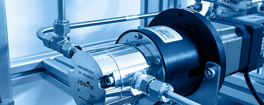
Rheology of Gear Pumps with Extreme High-Viscosity Fluids and Integrated Heat Tracing & Insulation Engineering
Abstract
When the working fluid's viscosity climbs from the MPa·s range into the Pa·s and even kPa·s range, the design logic of a gear pump undergoes a fundamental inversion. In low-viscosity duties every engineering effort is spent on suppressing clearance leakage; at extreme-high viscosity the clearance leakage becomes negligible (less than 0.005 % in the worked example), and the real bottlenecks shift to two severely under-rated links: whether the inlet can fully fill the tooth space, and whether the system can sustain the working temperature.
This white paper targets molten resins and polymers (EVA hot-melt adhesive, polyester polyol, epoxy resin prepolymer, PA / PET melt) as the primary objects, covering a viscosity envelope of 10 – 5 000 Pa·s and a temperature envelope of 80 – 220 °C, and establishes an engineering methodology coupling three fields — rheology, heat transfer and crystallisation kinetics:
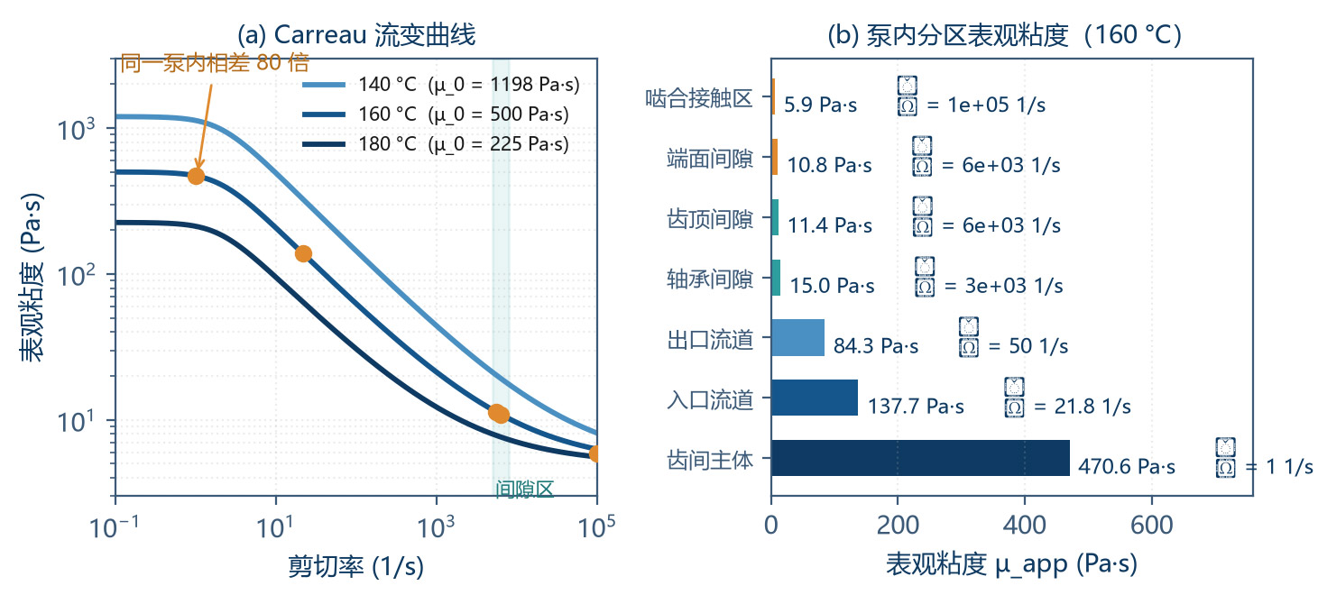
1Rheology layer: a gear pump internally spans a five-order-of-magnitude shear-rate spectrum (≈ 1 – 20 s⁻¹ in the tooth-space transport zone, ≈ 20 s⁻¹ in the inlet channel, 5 000 – 6 000 s⁻¹ in the tip / face clearance). The Carreau-model worked example shows that the same fluid in the same pump has apparent viscosities of 471 Pa·s in the stagnant zone, 138 Pa·s in the inlet, and only 11.4 Pa·s in the clearance zone — a 41× spread. Using a single viscosity value for the whole pump design is the most common and most dangerous simplification. Three region-matched apparent-viscosity design rules are given; the Nahme-Griffith number for the example is Na = 1.27 > 1, confirming strong flow–temperature coupling.
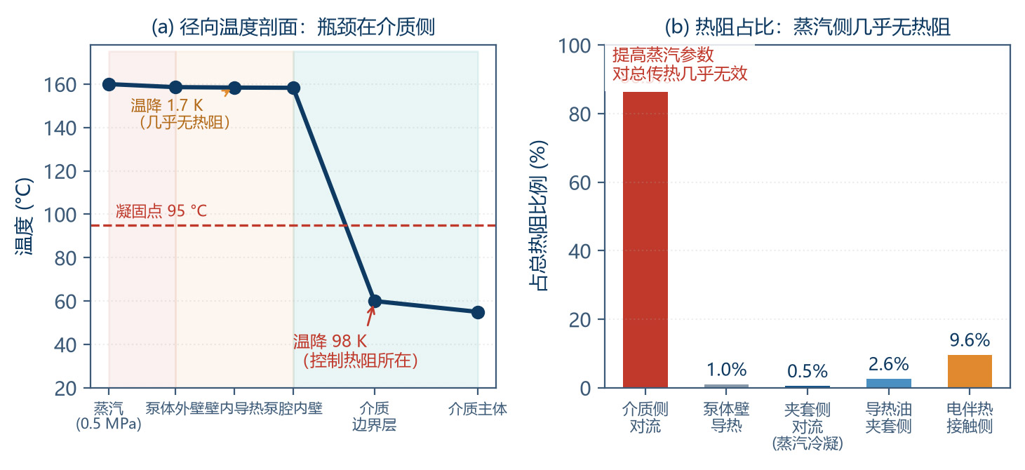
2Heat-transfer layer: a five-resistance thermal network is built (medium convection → body conduction → jacket convection → insulation → environment) and the bottleneck is quantified. The steam-side condensation coefficient (5 000 – 15 000 W/(m²·K)) contributes almost no resistance, while the high-viscosity medium side delivers only 36.6 W/(m²·K) — two orders of magnitude lower. The medium's thermal-diffusion time constant is -250 s, i.e. two orders of magnitude longer than the pump residence time (-1 – 2 s): the jacket can only "insulate + heat the thin near-wall layer", never heat a cold charge to working temperature. Nine-dimension coMParison matrices for steam vs self-regulating / constant-power / MI mineral-insulated electric tracing, critical radius and economic thickness of insulation, and a complete tracing-power sizing procedure are provided (example: 56 W steady-state, 510 W heat-up, 800 – 1 000 W design).
3Crystallisation-control layer: based on Avrami kinetics and Fourier-number thermal-diffusion analysis, a three-stage start-up sequence is established (pre-heat → soak → start). Two critical time constants are quantified: the metallic pump body's thermal balance time is only 39 s, while the medium's in-chamber soak time is 8 – 40 min — "the body is hot" does not imply "the medium is melted". Thermo-mechanical coupling is also quantified: a 20 K differential between body and gears produces an 8.6 µm radial-clearance change (22 % of the 40 µm design value), justifying the empirical heating-rate cap of 30 – 50 K/h.
The whole paper is threaded by a single worked example (22 mL/rev, 160 °C, 2.0 MPa, EVA hot-melt adhesive); Chapter 6 lays out the full 14-step engineering verification flow. Every numerical value can be re-checked with the formulas in the paper.
1 Introduction — The Design-Logic Inversion at Extreme-High Viscosity
1.1 A Paradigm Shift Driven by Viscosity
Liquid transport can be split into four regimes by viscosity. Each regime has its own governing equation and design focus. Understanding this partitioning is the prerequisite for avoiding the trap of "applying low-viscosity experience to a high-viscosity duty":
| Regime | Dynamic Viscosity Range | Typical Medium | Reynolds Number Re | Main Concern | Dominant Control of η_v |
|---|---|---|---|---|---|
| Low viscosity | 0.3 – 10 MPa·s | Solvents, water, monomers | 10³ – 10⁵ | Clearance leakage, cavitation | Clearance h³ and pressure difference |
| Medium viscosity | 10 – 1 000 MPa·s | Oils, coatings, photoresist | 10 – 10³ | Leakage and filling | Leakage / speed ratio |
| High viscosity | 1 – 100 Pa·s | Resins, syrups, inks | 10⁻² – 10 | Inlet filling, drive torque | Filling adequacy Φ |
| Extreme-high viscosity | 100 – 10⁵ Pa·s | Molten polymers, hot-melt adhesives, bitumen | 10⁻⁵ – 10⁻¹ | Filling + temperature + solidification | Temperature field & crystallisation state |
Table 1-1 Viscosity-based regime partitioning of fluids and the corresponding design focus
Table 1-1 delivers the central thesis of this paper: at extreme-high viscosity the Reynolds number drops to 10⁻⁵ – 10⁻¹, viscous forces dominate completely, and the inertia term can be neglected. This means:
Clearance leakage almost vanishes: the pressure-driven leakage term scales as h³/µ; a 1000× rise in µ drops leakage by 1000×. The example shows leakage share below 0.005 % and volumetric efficiency above 99.5 %.
Inlet filling becomes the sole bottleneck: whether the tooth space can be filled in the finite time it spends in the inlet region depends on the viscous filling rate — the most frequent failure mode of high-viscosity pumps.
Viscous friction torque explodes: the viscous term can exceed 20 – 40 % of the pressure term and grows non-linearly with speed.
Viscous dissipation becomes non-negligible: local shear heating can raise the medium by several Kelvin, coupling back into the temperature field.
Temperature is a life-or-death variable: once temperature drops below the solidification / melting point, the medium freezes and the pump is scrapped within tens of minutes.
1.2 Working Objects and Operating Envelope
| Medium | Operating T (°C) | Zero-shear viscosity µ_0 (Pa·s) | Melting / pour point (°C) | Rheology | Main Risk |
|---|---|---|---|---|---|
| EVA hot-melt adhesive | 150 – 180 | 200 – 800 | Tm = 75 – 95 | Strong shear-thinning, n ≈ 0.45 | Overtemp degradation, stop crystallisation |
| Polyester polyol | 80 – 120 | 5 – 50 | Pour point 10 – 30 | Near-Newtonian / weak shear-thinning | Moisture absorption, local overtemp |
| Epoxy prepolymer | 60 – 100 | 10 – 100 | Tg = −20 – 20 | Near-Newtonian, thixotropic | Overtemp cross-linking (irreversible) |
| PA hot-melt adhesive | 180 – 210 | 100 – 500 | Tm = 150 – 165 | Shear-thinning + high E_a | High melting point, narrow margin |
| PET melt | 270 – 290 | 100 – 400 | Tm = 255 – 265 | Shear-thinning, high E_a | High-temp degradation, carbonisation |
| Modified bitumen | 140 – 180 | 200 – 2 000 | Softening point 45 – 90 | Strong shear-thinning + thixotropy | Cooling hardening, coking |
| Silicone rubber / sealant | 25 – 80 | 500 – 5 000 | No clear melting point | Yield stress + strong shear-thinning | Very high start-up torque, air entrapment |
Table 1-2 Typical extreme-high-viscosity media and their process parameters
The worked example uses EVA hot-melt adhesive as the representative duty: operating temperature 160 °C, zero-shear viscosity 500 Pa·s, melting point 85 °C, viscous-flow activation energy 65 kJ/mol. It carries four diagnostic attributes simultaneously — high viscosity, strong shear-thinning, clear melting point and degradation risk — making it an ideal sample for validating the complete method.
1.3 Triple Challenge and Roadmap
The engineering difficulties of an extreme-high-viscosity gear pump can be summarised in three mutually coupled challenges:
① Challenge 1 (rheology): the medium is non-Newtonian, the shear-rate spectrum is extremely wide, and viscosity is highly temperature-sensitive. Using the wrong viscosity value can lead to inlet design failure or wrong motor selection.
② Challenge 2 (heat transfer): temperature must be maintained throughout the duty, but the residence time is short and the medium's conductivity is poor, so the tracing system must be precisely engineered — preventing both solidification and local over-degradation.
③ Challenge 3 (phase change): the crystallisation / solidification / re-melting cycle in stop-and-restart sequences is a dynamic game between thermal-diffusion time and mechanical clearance — the highest-failure-rate section in field practice.
Chapter 2 addresses Challenge 1; Chapter 3 addresses Challenge 2; Chapter 4 addresses Challenge 3; Chapter 5 gives the integrated engineering design method; Chapter 6 demonstrates the full 14-step verification flow with a worked example.
2 Non-Newtonian Rheology and the Shear-Stress Field
2.1 Rheological Model Spectrum — From Power Law to Carreau
To capture the constitutive behaviour of high-viscosity non-Newtonian fluids the appropriate model must be chosen by shear-rate range and whether a yield stress needs to be represented:
| Model | Constitutive Equation | Parameters | Strength | Limitation | Applicable γ̇ Range |
|---|---|---|---|---|---|
| Newtonian | τ = µ·γ̇ | µ | Simplest | Cannot describe shear-thinning | Narrow (Newtonian media) |
| Power-law (Ostwald) | τ = K·γ̇ⁿ | K, n | Simple, analytically tractable | Diverges at γ̇ → 0 (µ → ∞) and γ̇ → ∞ (µ → 0) | Moderate γ̇ (10 – 10³ s⁻¹) |
| Cross | µ = µ_∞ + (µ_0 − µ_∞) / [1 + (λγ̇)^(1−n)] | µ_0, µ_∞, λ, n | Two plateau limits, few parameters | Fit precision slightly below Carreau | Full range |
| Carreau | µ = µ_∞ + (µ_0 − µ_∞)·[1 + (λγ̇)²]^((n−1)/2) | µ_0, µ_∞, λ, n | Two clear plateau limits, best fit | More parameters, needs wide-range data | Full range (recommended) |
| Herschel–Bulkley | τ = τ_y + K·γ̇ⁿ | τ_y, K, n | Includes yield stress | Complex low-γ̇ behaviour | Filled systems |
| Bingham | τ = τ_y + µ_p·γ̇ | τ_y, µ_p | Yield + Newtonian plateau | No shear-thinning | Greases, pastes |
Table 2-1 Common rheological models and their applicable ranges
This paper recommends the Carreau model as the engineering main model. Three reasons: (1) it captures both the zero-shear plateau µ_0 (governing start-up torque and stagnant behaviour) and the infinite-shear plateau µ_∞ (governing the actual flow resistance in the gap); (2) the relaxation time λ directly gives the critical shear rate γ_c = 1/λ, a natural marker for splitting the rheological regions; (3) all parameters can be fitted directly from a steady-state sweep on a rotational rheometer.
| Parameter | Symbol | Value | Physical Meaning |
|---|---|---|---|
| Zero-shear viscosity | µ_0 | 500 Pa·s | Viscosity at rest or very low speed; governs start-up torque |
| Infinite-shear viscosity | µ_∞ | 5 Pa·s | Limit viscosity at extreme shear; governs clearance flow resistance |
| Relaxation time | λ | 0.5 s | Molecular-chain relaxation time; critical shear rate γ_c = 1/λ = 2 s⁻¹ |
| Power-law index | n | 0.45 | n < 1 indicates shear-thinning; 0.45 is strong shear-thinning |
| Density | ρ | 1 050 kg/m³ | — |
| Specific heat | c_p | 2 000 J/(kg·K) | — |
| Thermal conductivity | λ_th | 0.22 W/(m·K) | Very low; root cause of the heat-transfer bottleneck |
| Viscous-flow activation energy | E_a | 65 kJ/mol | Determines temperature sensitivity of viscosity |
Table 2-2 Carreau parameters of the example fluid (EVA hot-melt, 160 °C)
2.2 The Internal Shear-Rate Spectrum of a Gear Pump
This is the most critical insight of the chapter. A gear pump may be small but internally spans five orders of magnitude in shear rate. The shear rate at each location determines the actual viscosity of the medium there, which in turn governs the local physics:
| Location | Characteristic Speed (m/s) | Characteristic Gap (mm) | γ̇ (s⁻¹) | µ_app (Pa·s) | Governing Behaviour |
|---|---|---|---|---|---|
| Tooth-space transport (bulk) | 0.05 – 0.1 | 5 – 7 | 1 – 20 | 300 – 470 | Bulk transport, viscous drag |
| Inlet channel (pipe) | 0.068 | 25 (pipe Ø) | ≈ 22 | 138 | Inlet filling resistance |
| Outlet channel | 0.15 – 0.3 | 25 (pipe Ø) | ≈ 50 – 100 | 80 – 110 | Outlet pressure loss |
| Journal bearing clearance | 0.16 | 0.03 – 0.08 | 2 000 – 5 300 | 11 – 16 | Load capacity & friction loss |
| Tip / radial clearance | 0.22 | 0.04 | 5 500 | 11.4 | Radial leakage, clearance shear |
| Face / axial clearance | 0.157 | 0.025 | 6 280 | 10.8 | Axial leakage, viscous friction torque |
| Mesh-contact zone | 0.3 – 0.5 | 0.005 – 0.02 | 1.5×10⁴ – 1×10⁵ | ≈ 5.5 – 7 | Extreme shear; degradation risk |
Table 2-3 Internal shear-rate spectrum and the corresponding apparent viscosity (example: n = 100 r/min, m = 3 mm, z = 12, B = 30 mm)
The last column of the table is the core tool of this paper:
The ratio between maximum and minimum is 41×. This number demonstrates that any "design-with-one-viscosity-value" approach will fail in two opposite directions at once: if the low value (e.g. 11.4 Pa·s in the clearance zone) is used, the inlet design will be severely insufficient and the pump will simply starve; if the high value (471 Pa·s at rest) is used, drive torque and tracing power will be over-estimated several-fold, wasting resources or even leading to misjudgement.
2.3 Design Rule — Match Apparent Viscosity to Shear-Rate Region
| Design Task | Control Region | Adopt γ̇ | Example µ_app (Pa·s) | Consequence of Wrong Value |
|---|---|---|---|---|
| Clearance leakage check | Face / radial clearance | γ̇ = v/h, ≈ 5 000 – 6 500 s⁻¹ | 10.8 – 11.4 | Using 471 → leakage underestimated 40×, η_v misjudged |
| Inlet filling & suction | Inlet channel + tooth space | γ̇ = 8v/D, ≈ 10 – 50 s⁻¹ | 100 – 200 | Using 11.4 → inlet Δp underestimated 12×, pump starves |
| Drive torque & motor selection | Flank + face + bearing | γ̇ weighted, ≈ 3 000 – 6 000 s⁻¹ | 11 – 16 (shear term) | Using only shear value → cold-start torque severely underestimated |
| Bearing load & PV check | Journal bearing clearance | γ̇ = v/h_b, ≈ 2 000 – 5 300 s⁻¹ | 11 – 16 | Using 471 → friction loss overestimated, cooling design too conservative |
| Tracing power & residence | Pump chamber bulk | γ̇ ≈ 1 – 20 s⁻¹ | 300 – 470 | Using low value → natural convection overestimated, soak time underestimated |
| Shear degradation | Mesh-contact zone | γ̇ = 1.5×10⁴ – 10⁵ s⁻¹ | 5.5 – 7 (but τ high) | Ignoring high-γ̇ zone → chain scission, molecular weight loss |
Table 2-4 Apparent-viscosity selection rules for the three main design tasks
Special attention to the last row: low viscosity does not mean low shear stress. The mesh-contact zone has an apparent viscosity of only 5.5 Pa·s but a shear rate up to 10⁵ s⁻¹, so the shear stress τ = µ·γ̇ reaches 5.5 × 10⁴ = 55 kPa or higher, which is enough to cause mechanical degradation of long-chain polymers. For shear-sensitive media (high-MW PET, long-chain polyolefins) the high-shear peak should be suppressed by enlarging the clearance and reducing the speed, rather than looking at viscosity alone.
2.4 Temperature Effect on Viscosity — Arrhenius and WLF
High-viscosity media are far more temperature-sensitive than low-viscosity media. Two descriptions apply in different ranges:
2.4.1 Arrhenius Equation
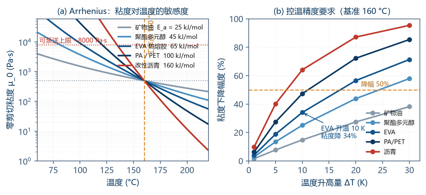
The viscous-flow activation energy E_a is the core parameter — the larger E_a, the more sensitive viscosity is to temperature. A more intuitive engineering form is the viscosity–temperature coefficient:
Example (E_a = 65 kJ/mol, T = 433 K): β = 65 000 / (8.314 × 433²) = 0.0417 K⁻¹, i.e. viscosity drops by 4.1 % per 1 K temperature rise, and by -34 % per 10 K rise.
| Medium | E_a (kJ/mol) | β @ Working T (K⁻¹) | Viscosity Drop for +10 K | Temperature-Control Demand |
|---|---|---|---|---|
| Mineral oil | 15 – 25 | 0.008 – 0.014 | 8 – 13 % | Routine ±5 °C |
| Polyester polyol | 30 – 45 | 0.017 – 0.026 | 16 – 23 % | ±3 °C |
| EVA hot-melt | 55 – 80 | 0.035 – 0.050 | 30 – 39 % | ±2 °C |
| PA hot-melt | 70 – 100 | 0.042 – 0.060 | 34 – 45 % | ±2 °C |
| PET melt | 80 – 120 | 0.045 – 0.068 | 36 – 49 % | ±1 – 2 °C |
| Modified bitumen | 120 – 200 | 0.070 – 0.115 | 50 – 68 % | ±1 °C |
Table 2-5 Viscous-flow activation energy & temperature sensitivity of typical media
This table gives the direct basis for the design of temperature-control accuracy: for bitumen-class media, +10 K already cuts viscosity by -60 %; with ±5 °C control the flow fluctuation can reach ±30 %, which is unacceptable in quantitative coating or metering duty. Therefore high-E_a media must be paired with high-precision temperature control (±1 – 2 °C).
2.4.2 WLF Equation
For amorphous polymers in the range Tg to Tg + 100 K, the Arrhenius equation fails and the WLF equation must be used:
With Tg as reference, the universal constants are C₁ = 17.44 and C₂ = 51.6 K. WLF's distinctive feature is that viscosity rises divergently as T approaches Tg — the medium transforms from fluid to glassy solid over a very narrow temperature window. This is the physical origin of the anti-crystallisation / solidification control discussed in Chapter 4.
2.5 Viscous Dissipation and the Nahme-Griffith Number
In high-viscosity flow, mechanical work is converted to heat by viscous dissipation. The local power density is:
The face-clearance shear is the dominant dissipation source. In the example: face shear stress τ = 10.8 × 6 280 = 67.8 kPa, face friction loss -19.6 W, tip -0.75 W, total -20.4 W. For 2 L/min throughput (ṁ = 0.035 kg/s):
Looking only at 0.29 K the effect seems negligible, but the danger of viscous dissipation is its positive feedback with the temperature field: local heating → viscosity drop → shear-stress drop (negative feedback, beneficial), but if the local temperature rises too high it triggers degradation (irreversible). The coupling strength is judged by the Nahme-Griffith number:
Substituting the example values (β = 0.0417 K⁻¹, µ = 138 Pa·s, v = 0.22 m/s, λ_th = 0.22 W/(m·K)):
Na > 1 means the temperature rise from viscous dissipation is large enough to significantly alter the local viscosity field; flow and temperature fields must be solved coupled. Engineering implication: an isothermal assumption cannot be used for flow prediction; the energy equation must be enabled in CFD, or 3 – 8 % flow-correction margin should be left in the design.
2.6 Thixotropy and Stop / Restart Behaviour
Filled resins, sealants and modified bitumen generally exhibit thixotropy: under constant shear the viscosity drops with time; on standing, the structure rebuilds and viscosity recovers. Use a structural parameter ξ (0 = fully broken, 1 = fully rebuilt):
where a is the structural-breakdown rate constant and b is the rebuild rate constant. The engineering problem brought by thixotropy is the viscosity hysteresis during a stop-and-restart cycle:
| Stop Duration | Structure Recovery ξ | Restart Viscosity (relative to continuous run) | Start-up Torque Multiplier | Engineering Countermeasure |
|---|---|---|---|---|
| < 5 min | 0.2 – 0.4 | 1.2 – 1.6 × | 1.2 – 1.6 × | Direct start acceptable |
| 5 – 30 min | 0.4 – 0.7 | 1.6 – 3 × | 1.6 – 3 × | Low-speed jog before start |
| 30 min – 4 h | 0.7 – 0.9 | 3 – 8 × | 3 – 8 × | Jacket pre-heat + jog |
| > 4 h | 0.9 – 1.0 | 8 – 20 × | 8 – 20 × | Full pre-heat → soak sequence (see Chapter 4) |
| Crystallised (below pour point) | — | Solid, no flow | ∞ (cannot start) | Must reheat above melt point and soak |
Table 2-6 Stop / restart effects of thixotropic media and countermeasures
Design must check against the "worst-case restart": the start torque of motor and transmission (including magnetic coupling) should be ≥ 2.5× the cold-start torque peak, and torque limiting with time-out protection must be configured to avoid stalling and burning out.
3 Heat-Transfer Mechanism & Efficiency of the Integrated Tracing Jacket
3.1 Multi-Layer Cylindrical Thermal-Resistance Network
The heat-transfer path of an integrated tracing jacket can be abstracted into five thermal resistances in series. Per unit length:
| # | Resistance | Expression | Physical Process | Example (K/W) | Share |
|---|---|---|---|---|---|
| R_in | Medium-side convection | 1 / (2π · r₁ · L · α_in) | Forced / natural convection, laminar, low Nu | 0.145 | 86.3 % |
| R_wall | Body-wall conduction | ln(r₂/r₁) / (2π · λ_wall · L) | Metal conduction, high λ | 0.0016 | 1.0 % |
| R_jacket | Jacket-side convection | 1 / (2π · r₂ · L · α_j) | Steam condensation / heat-transfer oil / heating-cable contact | 0.0008 (steam) | 0.5 % |
| R_ins | Insulation conduction | ln(r₄/r₃) / (2π · λ_ins · L) | Porous-medium conduction | — (in series with R_ext) | — |
| R_ext | Outer-surface conv. + radiation | 1 / (2π · r₄ · L · α_ext) | Natural convection in air + radiation | — | — |
Table 3-1 Definition and typical magnitude of each thermal-resistance term
The most striking number in Table 3-1 is R_in = 86.3 %. The efficiency of the tracing system is almost entirely determined by the medium-side convection; however well the jacket side is engineered, it cannot compensate.
3.2 Bottleneck Identification — Why the Medium Side Dominates
High-viscosity media have a very low convection coefficient, rooted in laminar flow and an extremely high Prandtl number.
3.2.1 Reynolds and Nusselt Numbers
Example (ρ = 1 050, v = 0.068 m/s, D_h = 0.025 m, µ = 138 Pa·s):
Re = 0.013 is creeping flow, where the inertia term is fully negligible. For fully developed laminar flow in a circular pipe the Nusselt number is a constant:
The corresponding convection coefficient:
3.2.2 CoMParison of Convection Coefficients at Each Side
| Position | Mechanism | α (W/(m²·K)) | Relative to Medium Side | Engineering Verdict |
|---|---|---|---|---|
| High-viscosity medium side | Creeping-flow laminar, conduction-dominated | 30 – 60 | 1× | Absolute bottleneck |
| Heat-transfer-oil jacket side | Forced convection (turbulent) | 500 – 2 000 | 17 – 67× | Not a bottleneck |
| Steam condensation side | Film condensation phase change | 5 000 – 15 000 | 167 – 500× | Effectively zero resistance |
| Heating-cable contact side | Contact conduction (with contact resistance) | 100 – 500 | 3 – 17× | Contact quality decides |
| Insulation outer surface | Natural convection in air + radiation | 10 – 25 | — | Decides heat loss |
Table 3-2 CoMParison of convection-coefficient orders along the heat-transfer path
The steam-side coefficient is 167 – 500× the medium side; raising steam pressure or steam flow has almost no effect on the overall heat transfer. This is the most common and most resource-wasting misconception in tracing engineering. Only three directions are effective:
enhance medium-side convection: exploit the mixing produced by gear meshing (a gear pump is better than a piston pump here), optimise the flow path so the near-wall layer is continuously refreshed, moderately raise the velocity;
shorten the heat-transfer path: design internal flow paths as thin layers, avoid thick-walled large-area "dead zones";
exploit shear-thinning: high-shear regions have low viscosity and locally better convection, so maintaining sufficient speed helps soak (but only up to the filling limit).
3.3 Residence Time vs Thermal-Diffusion Time — Functional Boundary
This is the fundamental criterion that defines the design objective of the tracing system.
3.3.1 Two Time Constants
Pump residence time:
Medium's thermal-diffusion time (with characteristic half-thickness L_c = 5 mm):
t_diff / t_res = 238 / 9 ≈ 26×. That is, in the time the medium spends inside the pump, heat can diffuse inward only about 1/26 of the characteristic distance (≈ 0.19 mm).
3.3.2 Functional Boundary of the Tracing Jacket
| Function | Feasible? | Physical Basis | Engineering Implication |
|---|---|---|---|
| Maintain medium temperature and compensate heat loss | √ Fully feasible | Heat loss only 15 – 60 W, tracing capacity far exceeds demand | Basic function of tracing |
| Heat the near-wall thin layer (< 1 mm) | √ Feasible | Heat-diffusion distance in residence time ≈ 0.2 – 1 mm | Lowers wall slip; improves start-up |
| Prevent wall crystallisation / solidification | √ Feasible | Wall temperature held above solidification point | Key measure against crystallisation |
| Heat cold medium to working temperature quickly | × Not feasible | t_diff is 26× t_res | Must be done by tank / pre-heater |
| Correct internal temperature non-uniformity | × Almost not feasible | Insufficient mixing time & space inside pump | Needs static mixer + line tracing |
| Compensate temperature drop at high flow | △ Limited | Constrained by residence time | Recompute tracing power by flow |
Table 3-3 Functional boundary of the tracing jacket — what it can and cannot do
The direct guidance to system design from this boundary: the tracing jacket is an "insulator" not a "heater". The cold-start heat duty must be supplied by tank heating, line tracing or a pre-heater. Placing the hope on the pump's jacket alone leads to start-up failure or an uncomfortable long "dry waiting".
3.4 Steam Tracing — Latent-Heat Characteristics & Engineering Keys
3.4.1 Steam Parameters and Their Temperature Correspondence
| Gauge Pressure (MPa) | Saturation Temperature (°C) | Latent Heat (kJ/kg) | Applicable Media | Note |
|---|---|---|---|---|
| 0.3 | 143.6 | 2 134 | Polyester polyol, epoxy prepolymer | Common low-pressure |
| 0.5 | 158.1 | 2 093 | EVA hot-melt | Common |
| 0.8 | 175.4 | 2 048 | EVA, PA (low-T segment) | Common high-pressure |
| 1.0 | 184.1 | 2 015 | PA hot-melt | — |
| 1.6 | 204.3 | 1 945 | High-melting-point resins | Requires special trap |
| 2.5 | 226.0 | 1 839 | Specialty high-temperature | Pump-body pressure rating must be checked |
Table 3-4 Saturated-steam pressure / temperature / latent heat lookup
The core advantage of steam tracing is phase-change isothermal. As long as two phases coexist inside the jacket, the wall temperature equals the saturation temperature for that pressure and does not drift with the heat load — naturally avoiding local over-heating. This is critical for heat-sensitive resins.
3.4.2 Steam-Mass Calculation
Example: Q_total = 510 W (heat-up duty), r = 2 093 kJ/kg (0.5 MPa):
3.4.3 Steam Traps — The Largest Failure Source
| Type | Working Principle | Strength | Limitation | Failure Mode | Maintenance Key |
|---|---|---|---|---|---|
| Float-ball (mechanical) | Ball rises / falls with liquid level | Large discharge, continuous drain, no steam leak | Bulky, freeze-sensitive, water-hammer sensitive | Ball damage → steam leak or blockage | Periodic screen cleaning |
| Thermodynamic (disc) | Dynamic pressure of steam vs condensate | CoMPact, water-hammer-resistant, cheap | Intermittent discharge, noisy, low-T leaks | Disc wear → steam leak | Annual disc replacement |
| Bimetal (thermostatic) | Bimetal strip bends with temperature | Adjustable drain T, freeze-resistant | Slow response, back-pressure sensitive | Fatigue → stuck open steam leak | Periodic calibration |
| Thermostatic bellows | Liquid in bellows vaporises & expands | Precise control, can run below saturation | Limited bellows life | Bellows damage → stuck open | 2 – 3 year replacement |
Table 3-5 Steam-trap selection & failure modes
Key tip: trap failure is the #1 fault of steam-tracing systems. Field statistics show that for systems in service more than 3 years the trap failure rate can reach 20 – 40 %. Steam leaks waste energy; blockage causes condensate accumulation, water hammer, and freeze-up in winter. Each tracing circuit must therefore have its own independent trap with a bypass, and be on a periodic inspection schedule.
3.5 Electric Tracing — Three Technology Routes
| Type | Structure & Principle | Max. Withstand T | Power Density | Control Accuracy | Best Use |
|---|---|---|---|---|---|
| Self-regulating heating cable | PTC conductive polymer; resistance rises with T → power drops | 65 – 135 °C (maintain) ≤ 205 °C (exposed) | 10 – 60 W/m | ±5 – 10 °C | Freeze protection, low-T pipe tracing, ≤ 120 °C resin hold |
| Constant-power heating cable | Parallel / series resistance wire, near-constant power | 150 – 260 °C | 10 – 100 W/m | ±2 – 5 °C (with controller) | Mid-T resin piping, stable output needed |
| MI mineral-insulated heating cable | MgO insulation + metal sheath (Inconel / 316L / Cu) | 400 – 600 °C | 10 – 200 W/m | ±1 – 3 °C (with SCR / PID) | PET / PA melt, high-T reactor discharge, > 200 °C specialty duty |
Table 3-6 CoMParison of three electric-tracing routes
A frequently overlooked detail in electric-tracing design is contact thermal resistance. If an air gap exists between the cable and the pump body / pipe wall, the heat-transfer coefficient drops from 500 to below 100 W/(m²·K). Engineering measures:
The cable must be wrapped with aluminium-foil tape or metal foil to enlarge the contact area and form a heat-spreading layer.
Use thermally conductive paste (λ = 0.7 – 2.0 W/(m·K)) to fill the air gaps on irregular surfaces.
In helical wrapping, keep the pitch 1.5 – 3× the tape width — too dense causes over-heating, too sparse causes non-uniformity.
MI cables can be pre-embedded in the jacket by casting — the minimum contact resistance, the first choice for high-T duty.
3.6 Steam vs Electric — Nine-Dimension Quantitative CoMParison
| Dimension | Steam Tracing | Electric (Self-reg / Const-power) | Electric (MI Cable) | Verdict |
|---|---|---|---|---|
| Max. temperature | Limited by boiler, usually ≤ 200 °C | ≤ 260 °C | ≤ 600 °C | MI > const-power > steam |
| Jacket-side α | 5 000 – 15 000 (condensation) | 300 – 500 (contact) | 300 – 500 (contact) | Steam wins (but not the bottleneck) |
| Temperature uniformity | Excellent (phase-change isothermal) | Fair (needs zoned control) | Good (high power density improves) | Steam wins |
| Control accuracy | ±5 – 10 °C (via pressure, coarse) | ±2 – 5 °C | ±1 – 3 °C | Electric wins |
| Response speed | Slow (boiler & line inertia, 30 – 120 min) | Fast (5 – 15 min) | Fast (3 – 10 min) | Electric wins |
| Energy-utilisation efficiency | 60 – 85 % (line loss, trap loss) | 92 – 97 % | 93 – 98 % | Electric wins |
| Initial investment | High (needs boiler / steam network) | Low to medium | High (custom + termination) | Self-reg wins |
| Operation & maintenance | High (trap, corrosion, winter freeze) | Low (periodic insulation check) | Very low (> 20-year life) | MI wins |
| Batch / intermittent adaptability | Poor (each start needs re-warming) | Excellent (instant on) | Excellent | Electric wins |
| 10-year TCO | Medium to high | Low to medium | Medium (high capex, low opex) | Depends on local energy cost |
Table 3-7 Steam vs electric tracing — quantitative coMParison matrix
Selection guidelines:
Large continuous plants with existing steam network and medium tolerating ±10 °C fluctuation → steam tracing (low energy cost, phase-change isothermal, naturally avoids local over-heating);
Distributed plants, intermittent operation, requiring ±2 – 5 °C precise control → self-regulating / constant-power electric tracing;
Working T > 200 °C, medium extremely sensitive to local over-heating, requiring > 20-year life → MI mineral-insulated cable + SCR + PID;
Thermosetting resins (epoxy, PU prepolymer) where over-temperature causes irreversible cross-linking → prefer electric tracing, because it allows multi-point monitoring and fast power-cut interlock, while steam systems are slow and cannot cut the heat input quickly.
3.7 Insulation — Critical Radius & Economic Thickness
3.7.1 Critical Insulation Radius
Adding insulation to a cylindrical wall shows a counter-intuitive behaviour: if the outer radius is smaller than a critical value, adding insulation actually increases the heat loss. The critical radius is:
Example (λ_ins = 0.045 W/(m·K), α_ext = 15 W/(m²·K)): r_c = 0.045/15 = 0.003 m = 3 mm. As long as the insulation outer diameter is greater than 3 mm (always true in practice), adding thickness always helps. The criterion is only meaningful for small-diameter piping and valves.
3.7.2 Economic Thickness & Outer-Surface Temperature Constraints
Engineering practice usually takes the outer-surface temperature constraint as the governing rule, rather than pure cost-optimality:
| Constraint | Requirement | Example Thickness (mm) | Resulting Heat-Loss Density | Applicable Scenario |
|---|---|---|---|---|
| Burn prevention (people-contact) | Outer T ≤ 50 °C | ≥ 45 | ≈ 45 W/m² | Personnel-access areas |
| Energy-saving standard | Heat-loss density ≤ 100 W/m² | ≥ 22 | ≈ 100 W/m² | General industry |
| High-E_a media T stability | Outer T ≤ 40 °C | ≥ 60 | ≈ 27 W/m² | Bitumen, PET melt |
| Freeze protection (extra time on trace failure) | Cool-down τ ≥ 8 h | ≥ 50 | — | Northern outdoor in winter |
| Example EVA at 160 °C | Outer T ≤ 45 °C | 50 | 36 W/m² | Used in this paper |
Table 3-8 Insulation-thickness design criteria (λ_ins = 0.045 W/(m·K), T_amb = 20 °C)
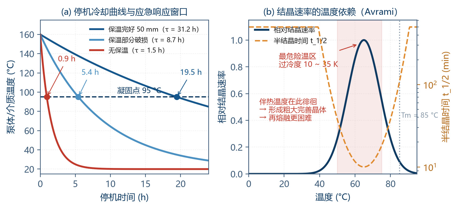
Worth highlighting is the "second function" of the insulation: it buys time when the tracing system fails. The example shows that with 50 mm aluminium silicate, the pump-body cool-down time constant is 31 h; going from 160 °C down to the solidification point 95 °C takes 19.5 h. With damaged insulation the same drop takes only -1 h. This gap decides the urgency of the fault response.
3.8 Complete Tracing-Power Sizing Procedure
The total tracing-power demand has three components:
| Component | Formula | Value | Note |
|---|---|---|---|
| ① Body heat-up | Q₁ = m · c · ΔT / t = 25 × 500 × 140 / 3 600 s | 486 W | Heat-up rate per hour |
| ② Medium heat-up | Q₂ = m_med · c_p · ΔT / t = 0.315 × 2 000 × 140 / 3 600 | 24 W | About 0.3 L in chamber |
| ③ Steady-state loss (insulated) | Q₃ = ΔT / R_ins = 140 / 8.99 | 15.6 W | 50 mm aluminium silicate |
| ④ Cold-spot extra loss | Flanges + supports + instrument ports | ≈ 40 W | Empirical; verify point by point |
| ⑤ Subtotal (steady) | ③ + ④ | 56 W | — |
| ⑥ Subtotal (heat-up) | ① + ② + ⑤ | 566 W | — |
| ⑦ Design margin | × 1.5 – 2.0 | 850 – 1 130 W | Aging, voltage variation, extreme environment |
| ⑧ Selection | — | 1 000 W (steam -2.0 kg/h; electric 1 000 W) | Includes all margins |
Table 3-9 Tracing-power calculation (example: 25 kg body, carbon steel, 160 °C, ambient 20 °C)
4 Engineering Thermodynamic Control against Start-Up Crystallisation
4.1 Thermodynamic Basis of Crystallisation and Solidification
The "loss-of-flow" behaviour of resins and polymers on cooling falls into three classes by molecular structure, each with a very different engineering response:
| Type | Example | Characteristic T | DSC Signature | Reversibility | Criterion |
|---|---|---|---|---|---|
| Semi-crystalline polymer (melt crystallisation) | EVA, PA, PET, PP, PE, POM | Melting point Tm | Sharp exothermic crystallisation peak on cooling; sharp endothermic melting peak on heating | Reversible (re-melt above Tm) | T_operate ≥ Tm + 30 K |
| Amorphous polymer (glass transition) | PS, PC, PMMA, uncured epoxy, rosin ester | Glass-transition Tg | No crystallisation peak; only a baseline step (specific-heat jump) | Reversible (softens above Tg) | T_operate ≥ Tg + 60 K, or back-calculate from viscosity cap |
| Oils / mixtures (pour-point solidification) | Modified bitumen, heavy oil, wax blend | Pour point, cloud point, softening point | Broad-temperature diffuse exotherm | Partially reversible (wax needs higher T and time) | T_operate ≥ pour point + 40 K |
Table 4-1 Three "loss-of-flow" mechanisms and identification
Identification is simple but often skipped: run a cooling–heating DSC. A sharp crystallisation peak + melting peak → treat as semi-crystalline; only a baseline step → treat as amorphous. This one experiment determines the temperature-margin rule for everything that follows; spending half a day on it is worthwhile.
4.2 Crystallisation Kinetics — The Avrami Equation
Crystallisation is not instantaneous; its progress follows the Avrami equation:
where X is the relative crystallinity, k the strongly temperature-dependent rate constant and n the Avrami index (1 – 4 depending on nucleation and growth dimensionality).
The key is the temperature dependence of k: the crystallisation rate has a maximum between Tg and Tm (typically near 0.8·Tm in Kelvin). Near Tm the thermodynamic driving force (under-cooling) is too small to nucleate; near Tg chain-segment motion is frozen and diffusion is rate-limiting; between them (≈ 0.8·Tm) driving force and diffusion reach the optimum balance and crystallisation is fastest.
| Temperature (°C) | Under-cooling ΔT = Tm − T (K) | Relative Crystallisation Rate | Half-crystallisation Time t₁/₂ | Engineering Meaning |
|---|---|---|---|---|
| 82 (ΔT = 3 K) | 3 | 0.02 | ≈ 500 min | Near melting point; almost no crystallisation |
| 75 (ΔT = 10 K) | 10 | 0.35 | ≈ 28 min | Slow-crystallisation zone |
| 65 (ΔT = 20 K) | 20 | 1.00 (fastest) | ≈ 10 min | Most dangerous temperature window |
| 50 (ΔT = 35 K) | 35 | 0.55 | ≈ 18 min | Crystallisation rate falls |
| 30 (ΔT = 55 K) | 55 | 0.18 | ≈ 55 min | Diffusion-limited |
| 0 (ΔT = 85 K) | 85 | 0.05 | ≈ 200 min | Near Tg; almost frozen |
Table 4-2 Temperature dependence of crystallisation rate (example: EVA, Tm = 85 °C = 358 K)
This table reveals a counter-intuitive but critical engineering fact: the most dangerous temperature window is not the coldest, it is the band just below the melting point (under-cooling 15 – 30 K). Two design lessons follow:
During a controlled cool-down the medium "passes through" the dangerous band. If cooling is fast (full tracing failure with no insulation), the medium drops below Tg before crystals have grown appreciably, forming a glassy solid that re-melts more easily.
If the medium "lingers" in the dangerous band (intermittent tracing, temperature swings), coarse well-formed crystals develop, which need higher temperature and longer time to re-melt. Hence the stability of the tracing system is more important than its power.
4.3 Operating-Temperature Margin Design Rules
| Medium Type | Reference Temperature | Recommended Margin | Example Value | Rationale |
|---|---|---|---|---|
| Semi-crystalline polymer | Tm (melting point) | T_operate ≥ Tm + 30 K | 85 + 75 = 160 °C | Avoid the crystallisation band; ensure full melt |
| Amorphous polymer | Tg (glass transition) | T_operate ≥ Tg + 60 K | — | Sufficient chain-segment mobility |
| Amorphous (viscosity-limited) | T_µmax (T at which µ reaches cap) | T_operate ≥ T_µmax + 15 K | — | Back-calculated from puMPable-viscosity cap |
| Oils / mixtures | Pour point or softening point | T_operate ≥ pour point + 40 K | — | Avoid wax precipitation & structure build-up |
| Thermosetting system | Reaction start T_react | T_operate ≤ T_react − 30 K | — | Upper-bound constraint; prevent cross-linking |
Table 3-8 (in Chapter 3 — repeated) — Operating-temperature margin design rules
Note the last row: for thermosetting systems (epoxy, PU prepolymer, phenolic) the constraint is an upper bound, not a lower one. Over-temperature in these media causes irreversible cross-linking; once cured inside the pump, the whole pump is scrapped. Such systems therefore require a dedicated high-temperature interlock (see §4.8).
4.4 Three-Stage Start-Up Sequence — Pre-heat → Soak → Start
This is the most operationally valuable section of the chapter. Many start-up failures in the field come from confusing "the body is hot" with "the medium is melted".
4.4.1 Two Time Constants with a Huge Gap
Metallic pump-body thermal balance time (half-thickness L = 30 mm, carbon steel a = 1.15 × 10⁻⁵ m²/s):
In-chamber medium soak time (characteristic half-thickness L_c = 10 mm, a_th = 1.05 × 10⁻⁷ m²/s):
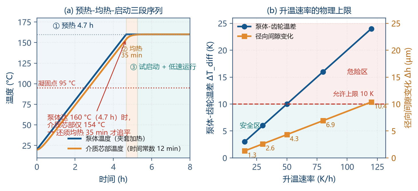
39 s vs 8 min — a 12× gap. With the medium at rest, pure conduction needs 8 min; natural convection induced by the temperature difference can accelerate 2 – 5×, so the engineering soak time is 20 – 40 min.
| Stage | Goal | Action | Criterion | Duration | Forbidden |
|---|---|---|---|---|---|
| ① Pre-heat | Body & jacket reach working T | Turn on tracing, ramp ≤ 30 K/h; inlet / outlet valves closed or slightly open | Body surface ≥ 150 °C and ramp rate met | ≈ 4.5 h (20 → 160 °C) | Rapid heat-up (> 60 K/h); starting the pump at this point |
| ② Soak | Chamber medium fully melted & temperature uniform | Hold tracing T; intermittent manual jog every 10 min (¼ turn) | Fo ≥ 0.5 and outlet/body ΔT ≤ 3 K | 20 – 40 min | Motor start; "body is hot so start now" |
| ③ Trial start | Confirm no seizure; flow established | Inching 2 – 3 times (1 – 2 s each); watch current & outlet P | Start-current peak ≤ 2.5× rated; outlet P stable | 1 – 2 min | Continuous start > 3 times; starting under pressure |
| ④ Warm-run | Stable flow & temperature field | Run at 20 – 30 % rated speed | Outlet P stable, no abnormal noise, current below rated | 5 – 15 min | Immediately ramping to rated speed |
| ⑤ Ramp to rated | Reach normal production | Ramp at 10 %/min | All parameters normal | — | — |
Table 4-4 Pre-heat → soak → trial → warm-run → ramp sequence (example: EVA, 160 °C)
4.5 Thermo-Mechanical Coupling — Differential Clearance Drift
This is a unique risk for precision gear pumps at extreme-high viscosity: body and gears do not warm up in synchrony, which dynamically changes the clearance.
4.5.1 Quantifying the Clearance Change
If body and gears are the same material (α = 12×10⁻⁶ K⁻¹), with a differential ΔT_diff:
| Body–Gear ΔT_diff (K) | Clearance Change Δh (µm) | Actual Clearance (µm) | Relative Change | Verdict |
|---|---|---|---|---|
| 2 (steady normal) | 0.9 | 40.9 | +2.2 % | Normal |
| 5 | 2.2 | 42.2 | +5.5 % | Normal |
| 10 | 4.3 | 44.3 | +11 % | Acceptable boundary |
| 20 | 8.6 | 48.6 / 31.4 | ±22 % | Danger: seizure or leakage surge |
| 30 | 13.0 | 53.0 / 27.0 | ±32 % | Certain failure |
| ≥ 40 | ≈ 17.3 | — | ±43 % | Bearing seizure or severe wear |
Table 4-5 Effect of differential temperature on radial clearance (D = 36 mm, design clearance 40 µm)
Note: the direction of the differential decides the consequence. If the gear is hotter than the body (gears expand more), clearance decreases — risk is seizure and bearing lock-up. If the body is hotter than the gear, clearance increases — risk is leakage surge and volumetric efficiency collapse. At start-up the body usually heats first (jacket heats body), so the second case is more common; at shut-down if the medium is still hot while the jacket is off, the first case can occur.
4.5.2 Physical Upper Bound on the Heat-Up Rate
The gear's temperature response lags the body's, with time constant:
Example (gear 0.5 kg, c = 460 J/(kg·K), h_eff = 50 W/(m²·K), A = 0.008 m²):
ΔT_diff ≈ (dT/dt) · τ_lag. Inverting this for the allowed heat-up rate:
| Heat-Up Rate (K/h) | Steady ΔT_diff (K) | Clearance Change (µm) | Verdict | Applicable Object |
|---|---|---|---|---|
| 15 | 2.4 | 1.0 | Excellent | Precision gear pumps (clearance < 30 µm) |
| 30 | 4.8 | 2.1 | Good (recommended) | Precision gear pumps, crystallising media |
| 50 | 8.0 | 3.5 | Acceptable | Conventional gear pumps |
| 80 | 12.8 | 5.5 | Critical | Only coarse pumps with clearance > 60 µm |
| 120 | 19.2 | 8.3 | Not acceptable | Forbidden for gear pumps |
| Sudden steam shock | > 30 | > 13 | Certain failure | Absolutely forbidden |
Table 4-6 Physical upper bound on heat-up rate (τ_lag = 9.6 min, allowed ΔT_diff ≤ 10 K)
This calculation provides the quantitative basis for the engineering rule of thumb "30 – 50 K/h". For precision gear pumps with clearance < 30 µm it should be tightened further to 15 – 30 K/h.
4.6 Cold-Spot Identification & Elimination
"Cold spots" are the localised regions of the tracing system that run significantly below the bulk temperature — the birthplace of crystallisation blockage.
| Cold-Spot Location | Cause | T Drop | Risk Level | Elimination |
|---|---|---|---|---|
| Inlet / outlet flanges | Large metal mass, large area, often uninsulated | 15 – 40 K | High | Flange tracing ring + removable insulation; minimise flange thickness |
| Safety / relief valve port | Thin branch pipe, no tracing, static medium | 25 – 60 K | Very high (static medium will solidify) | Tracing + shorten branch; or use diaphragm-type; or inert-liquid seal |
| Pressure / sensor port | Same as above; the sense cavity is stagnant | 20 – 50 K | High | Use diaphragm-sealed sensor with tracing; or silicone-oil pressure transmission |
| Pump-body support feet / base | Thermal-bridge effect; metal conducts heat to foundation | 10 – 30 K | Medium | Add insulation pad (ceramic fibre / epoxy board); reduce contact area |
| Insulation joints / openings | Construction defect; not restored after maintenance | 20 – 50 K | High | Double-layer offset wrapping; mandatory check after maintenance |
| Drain / sample valve | Dead leg; fully stagnant | 30 – 70 K | Very high | Eliminate where possible; if retained, individual tracing + trace to main pipe |
| Mechanical-seal / flush line | Thin pipe, no tracing | 20 – 45 K | Medium-high | Trace with main; shorten pipe length |
Table 4-7 Typical cold-spot inventory & elimination measures
The most effective cold-spot management tool is infrared thermography inspection. It is recommended to do a full thermographic scan at new-unit commissioning and after every maintenance, build a baseline map, and then inspect every quarter. Any point running more than 15 K below the bulk should be logged and corrected.
4.7 Shut-Down Protection Strategy
| Shut-Down Duration | Recommended Strategy | Operation Key Points | Re-Start Preparation |
|---|---|---|---|
| < 30 min | Hold tracing; do nothing | Tracing holds; pump body T does not drop | Direct start (low speed → rated) |
| 30 min – 4 h | Hold tracing | Tracing holds; close outlet valve to prevent back-flow | Low-speed trial; watch current |
| 4 – 24 h | Hold tracing (preferred) or flush | If tracing must stop, flush with low-viscosity coMPatible medium | Three-stage sequence: pre-heat → soak → start |
| 1 – 7 days | Flush + cool down | Flush with coMPatible solvent / low-viscosity oil; after cooling, switch off tracing | Re-fill with working medium then pre-heat |
| > 7 days / long-term | Flush + drain + inert-gas blanket | Fully drain; for oxidisable media blanket with nitrogen | Full start-up sequence + first-run inspection |
| Unplanned shut-down (tracing failure) | Emergency insulation + rapid restoration | Immediately enable backup tracing or temporary electric tracing; record the cooling curve | If crystallised, must strictly execute the soak procedure |
Table 4-8 Shut-down protection strategy by duration
A practical quantitative tool: the cooling time constant determines the emergency-response window:
| Insulation State | R_total (K/W) | τ_cool | Time to Drop to 95 °C (Solidification Point) | Response Requirement |
|---|---|---|---|---|
| Intact (50 mm) | 8.99 | 31.2 h | 19.5 h | Comfortable; next-day handling |
| Partially damaged | ≈ 2.5 | 8.7 h | 5.4 h | Must restore within shift |
| No insulation | ≈ 0.42 | 1.5 h | 58 min | Must restore within 1 h |
| No insulation + outdoor in winter | ≈ 0.30 | 1.0 h | 40 min | Immediate response, otherwise must drain |
Table 4-9 Cool-down time constants & emergency-response windows
4.8 Over-Temperature Interlock for Thermosetting Systems
For epoxy prepolymer, PU prepolymer and phenolic resin, over-temperature causes irreversible cross-linking. The cure rate follows Arrhenius:
Typical rule: each +10 K approximately doubles the cure rate. The design criterion is therefore:
| Item | Requirement | Implementation | Note |
|---|---|---|---|
| Upper-temperature setting | T_max ≤ T_react − 30 K | Tracing system setting + independent limit thermostat | T_react from DSC exotherm onset |
| Residence-time limit | SF_cure ≥ 10 | Verify against chamber volume and minimum flow | Low-flow duty is the highest risk |
| Independent high-T interlock | Hard-wired, not via PLC | Bimetal temperature switch → contactor open | Must be independent of control system |
| Post-over-temperature handling | Immediate drain + solvent flush | Emergency operating procedure | Once cross-linked, no remedy |
| Low-flow protection | Below threshold, derate or stop | Flow meter + interlock | Prevents "stagnation heating" |
Table 4-10 Temperature safety design for thermosetting systems
Key tip: the most dangerous operating condition for a thermosetting system is not "high temperature" alone but the combination "high T + low flow + long residence". This combination is most likely to occur during commissioning, standby and small-batch production; the control logic must specifically include a low-flow derating protection.
5 Integrated Engineering Design
5.1 Body–Jacket–Insulation Integrated Structure
The traditional approach "pump body + add-on jacket + field-wrapped insulation" has three drawbacks: large interface thermal resistance, many cold spots, and difficult restoration after maintenance. Integrated design treats the three as a whole:
| Layer | Design Content | Key Technologies | Effect |
|---|---|---|---|
| Layer 1 — Jacket body | Cast / welded jacket integrally formed with the body | Guide baffles inside jacket for forced spiral flow; uniform cavity thickness; diagonal inlet / outlet to avoid short-circuit | Eliminates interface resistance; jacket-side α up 30 – 60 % |
| Layer 2 — Flow-path optimisation | Short, large-diameter, no dead legs | L/D ≤ 5; minimise drain dead legs; integral flanges (reduce flange count) | Eliminates cold spots; reduces holdup & degradation risk |
| Layer 3 — Insulation enclosure | Factory-prefabricated moulded insulation shell | Moulded aluminium-silicate / nano-aerogel shell; removable with clamp; outer stainless / Al-foil cover | 100 % restoration after maintenance; uniform outer T; heat loss down 20 – 40 % |
Table 5-1 Three layers of the integrated tracing structure
Insulation-material selection deserves a separate discussion:
| Material | λ (W/(m·K)) @ 200 °C | Max. Use T | Density (kg/m³) | Strength | Limitation |
|---|---|---|---|---|---|
| Aluminium-silicate fibre | 0.09 – 0.13 | 1 000 °C | 128 – 200 | High T-tolerance, cheap, mature | Dust; performance drops when wet |
| Rock wool / slag wool | 0.07 – 0.10 | 600 °C | 100 – 160 | Cheap, non-combustible | Absorbs water, settles, limited T-tolerance |
| Nano-aerogel blanket | 0.020 – 0.028 | 650 °C | 180 – 220 | Lowest λ; thickness halved | Expensive (5 – 10×); degrades under compression |
| Microporous calcium silicate | 0.06 – 0.09 | 650 °C | 220 – 260 | Strong, mouldable | Heavy, brittle |
| Foam glass | 0.06 – 0.08 | 430 °C | 120 – 180 | Non-absorbent, corrosion-resistant | Limited T-tolerance, brittle |
| PU foam | 0.025 – 0.035 | 120 °C | 40 – 60 | Low λ, light, cheap | Low T-tolerance; only for low-T lines |
Table 5-2 Insulation material coMParison
For 160 – 220 °C resin duty, nano-aerogel blanket is the overall best choice: to reach the same outer-surface temperature the thickness drops from 50 mm to 20 – 25 mm, valuable in space-constrained pump skids; although the unit price is 5 – 10× higher, the long-term energy saving and half-thickness layout convenience typically make the total cost of ownership lower.
5.2 Tiered Temperature-Control Architecture
| Level | Controlled Variable | Control Mode | Measurement Point | Accuracy | Function |
|---|---|---|---|---|---|
| L1 Master | Medium outlet T | PID (master) | Outlet pipe, insertion ≥ 1/3 pipe Ø | ±1 – 2 °C | Core variable determining product quality |
| L2 Slave | Jacket / tracing-medium T | PID (slave, cascade) | Jacket inlet / outlet | ±3 °C | Fast suppression of heat-source disturbance |
| L3 Limit | Pump body surface T | Limit (does not regulate) | Body-surface thermocouple | ±5 °C | Prevents wall over-T → degradation |
| L4 Feedforward | Ambient T, flow | Feedforward compensation | Ambient sensor, flowmeter | — | Compensates seasonal & load variation |
| L5 Interlock | Over-T / low-T / low-flow | Hard-wired switch | Independent T-switch | — | Safety; independent of PLC |
Table 5-3 Tiered temperature-control architecture
Two extremely common mistakes:
Using jacket temperature as the master variable: this produces the illusion of "surface hot, inside cold". The jacket temperature being stable at the setpoint does not mean the medium has reached the working temperature, especially during start-up. The master variable must be the medium temperature.
Insufficient thermocouple insertion depth: high-viscosity media have very low conductivity; if the insertion depth is too shallow the measurement actually reflects the pipe-wall temperature rather than the bulk. Insertion ≥ 1/3 pipe Ø is required, with the sensing element located in the centre of the flow.
5.3 Anti-Condensation Design of Instruments & Sample Ports
Pressure gauge: prefer a diaphragm-sealed gauge with tracing (diaphragm contacts the medium, capillary filled with silicone oil for pressure transmission) — eliminates the impulse-line blockage problem.
Temperature sensor: use thermowell-protected RTD / thermocouple, sufficient insertion depth, thermally conductive silicone grease between well and medium to reduce contact resistance.
Safety valve: must trace up to the valve body; for media prone to crystallisation, use "rupture disc + safety valve in series" or "diaphragm-type safety valve" with pressure monitoring in between.
Sample port: design as a "refluxing sample loop" rather than a dead leg; sample can return to the system, avoiding dead-leg solidification.
Level / pressure switches: use flange-mounted direct-contact installation where possible, avoiding impulse lines.
5.4 Design Verification Checklist
| # | Check Item | Criterion | Reference Section |
|---|---|---|---|
| 1 | Rheology parameters acquired | Full γ̇ range 10⁻¹ – 10⁵ s⁻¹ viscosity curve at ≥ 3 temperatures | 2.1 |
| 2 | Shear-rate spectrum calculated | γ̇ and corresponding µ_app computed for tooth-space / inlet / clearance / mesh zones | 2.2 |
| 3 | Inlet filling check | Filling adequacy Φ ≥ 3; inlet pressurisation capability confirmed | 6.3 |
| 4 | Maximum speed determined | n ≤ n_max (back-calculated from Φ) with 30 % margin | 6.3 |
| 5 | Drive torque check | Includes pressure term + viscous term + cold-start term (× 2.5 safety factor) | 2.3 / 6.4 |
| 6 | Viscous dissipation evaluation | Compute Na; if Na > 1, coupled solution or margin needed | 2.5 |
| 7 | Leakage & volumetric efficiency | Check with clearance-zone µ_app; for high-viscosity should be > 99 % | 6.5 |
| 8 | Degradation risk evaluation | Mesh-zone shear stress < medium critical degradation stress; residence time limited | 2.3 |
| 9 | Thermal-resistance & bottleneck identification | Each resistance share quantified; medium side confirmed as control | 3.1 / 3.2 |
| 10 | Residence time vs thermal diffusion | Confirmed tracing is "insulation"; heating done by upstream system | 3.3 |
| 11 | Tracing power selection | Includes heat-up + loss + cold spots + margin; steam or electric form chosen | 3.8 |
| 12 | Insulation design | Outer r > critical radius; outer T meets constraint; cool-down τ known | 3.7 |
| 13 | Start-up sequence design | Pre-heat / soak / start three stages written into SOP; heat-up rate ≤ 30 – 50 K/h | 4.4 |
| 14 | Shut-down & interlock | Shut-down protection strategy clear; thermosetting systems have independent high-T interlock | 4.7 / 4.8 |
Table 5-4 14-step design verification checklist for extreme-high-viscosity gear-pump systems
6 Engineering Worked Example — Full Verification Procedure
6.1 Design Inputs
| Item | Symbol | Value | Unit |
|---|---|---|---|
| Medium | — | EVA hot-melt adhesive | — |
| Operating temperature | T_op | 160 | °C |
| Melting point | Tm | 85 | °C |
| Zero-shear viscosity | µ_0 | 500 | Pa·s |
| Infinite-shear viscosity | µ_∞ | 5 | Pa·s |
| Relaxation time | λ | 0.5 | s |
| Power-law index | n | 0.45 | — |
| Viscous-flow activation energy | E_a | 65 | kJ/mol |
| Density / sp. heat / conductivity | ρ / c_p / λ_th | 1 050 / 2 000 / 0.22 | kg/m³ / J/(kg·K) / W/(m·K) |
| Displacement | q | 22 | mL/rev |
| Geometry | m / z / B | 3 / 12 / 30 | mm / — / mm |
| Face / radial clearance | h_a / h_r | 25 / 40 | µm |
| Speed | n | 100 | r/min |
| Pressure difference | Δp | 2.0 | MPa |
| Inlet pressurisation | Δp_in | 0.90 | MPa |
| Ambient temperature | T_amb | 20 | °C |
Table 6-1 Worked-example design inputs
6.2 Rheology Calculation
| Zone | γ̇ (s⁻¹) | (λγ̇)² | µ_app (Pa·s) | Used for |
|---|---|---|---|---|
| Tooth-space bulk | 1 | 0.25 | 470.6 | Residence time, natural convection |
| Inlet channel | 21.8 | 118.8 | 137.7 | Inlet Δp, filling |
| Outlet channel | 50 | 625 | 84.3 | Outlet pressure loss |
| Bearing clearance | 3 000 | 2.25×10⁶ | 15.0 | Load, friction loss |
| Tip clearance | 5 500 | 7.56×10⁶ | 11.4 | Radial leakage |
| Face clearance | 6 280 | 9.86×10⁶ | 10.8 | Axial leakage, viscous torque |
| Mesh-contact zone | 100 000 | 2.5×10⁹ | 5.9 | Degradation risk evaluation |
| Max / min ratio | — | — | 470.6 / 5.9 = 80× | Single value cannot be used |
Table 6-2 Region-matched apparent viscosity results
6.3 Inlet Filling & Maximum Speed
Inlet pipe pressure drop (laminar Poiseuille, D = 25 mm, L = 1.5 m, v = 0.068 m/s, µ = 137.7 Pa·s):
Adding filter + local resistance 0.18 MPa gives total inlet demand 0.90 MPa — far beyond any gravity head (3 m head only 0.03 MPa); nitrogen pressurisation or feed-pump pressurisation must be configured.
Filling-time check: tooth-space volume V_t = q / (2z) = 22/24 = 0.917 mL; differential-driven fill velocity v_fill ≈ 0.40 m/s; flow area A = 2.025×10⁻⁴ m²:
Back-calculating the maximum speed (setting Φ = 3):
If inlet pressurisation drops from 0.90 to 0.30 MPa, v_fill drops to 1/3 and n_max drops to -148 r/min. The inlet pressurisation capability directly determines the maximum usable speed — a chain constraint that is most often overlooked in high-viscosity selection.
6.4 Drive Torque
| Component | Formula | Value (N·m) | Share | Note |
|---|---|---|---|---|
| Pressure torque | T_p = Δp · q / (2π) = 2.0×10⁶ × 22×10⁻⁶ / 6.283 | 7.00 | 68.6 % | — |
| Face viscous torque | τ = µ · γ̇ = 10.8 × 6 280 = 67.8 kPa; F = τ · A = 67.8×10³ × 1.626×10⁻³ = 110.2 N; T = F · r_m = 110.2 × 0.017 | 1.87 | 18.3 % | — |
| Tip viscous torque | F = 62.7 kPa × 5.4×10⁻⁵ = 3.39 N; T = 3.39 × 0.021 | 0.07 | 0.7 % | — |
| Bearing friction | Empirical | 0.50 | 4.9 % | — |
| Total (rated duty) | — | 9.44 | 100 % | — |
| Motor power | P = T · ω = 9.44 × 10.47 | 98.8 W | — | — |
| Motor selection | 1.5× margin + efficiency loss | 0.75 kW | — | — |
| Cold-start torque check | After thixotropy recovery µ ≈ 8× → viscous term × 8 | 22.5 N·m | — | Must be satisfied by motor & drive |
Table 6-3 Drive-torque breakdown
6.5 Leakage & Volumetric Efficiency
This result confirms the central judgement of Chapter 1: in extreme-high-viscosity duty leakage is no longer the design contradiction — filling and temperature are.
6.6 Tracing System
Following the procedure in §3.8: steady-state loss 56 W, heat-up demand 566 W, design margin 1.8× → selection 1 000 W.
| Option | Configuration | Capex | Opex Estimate | T Uniformity | Response | Recommendation |
|---|---|---|---|---|---|---|
| A — Steam | 0.5 MPa saturated steam, float-ball trap, -2.0 kg/h | Medium (needs network) | By steam price | Excellent | Slow | ★★★★☆ (when network exists) |
| B — Self-regulating | 40 W/m × 25 m, Al-foil tape | Low | By electricity price | Fair | Fast | ★★★☆☆ (max 135 °C, margin insufficient) |
| C — MI cable (recommended) | MI cable pre-embedded in jacket, SCR + PID | High | By electricity price | Good | Fast | ★★★★★ (recommended) |
| D — Heat-transfer oil | Dedicated oil unit + jacket circulation | High | Medium | Excellent | Medium | ★★★★☆ (centralised multi-pump heat) |
Table 6-4 Tracing options coMParison & selection
6.7 Start-Up Sequence
| Stage | Duration | Temperature State | Action | Completion Criterion |
|---|---|---|---|---|
| Pre-heat | 4.7 h (20 → 160 °C, 30 K/h) | Body 160 °C, medium core still cold | Turn on tracing | Body surface ≥ 150 °C |
| Soak | 35 min | Medium core approaches 160 °C | Hold T; manual jog ¼ turn every 10 min | Outlet / body ΔT ≤ 3 K |
| Trial start | 2 min | 160 °C | Inch 3 times | Current peak ≤ 2.5× rated |
| Warm-run | 10 min | 160 °C | 30 % speed | Pressure stable, no noise |
| Ramp to rated | 7 min | 160 °C | 10 %/min ramp | Parameters normal |
| Total | ≈ 5.9 h | — | — | — |
Table 6-5 Worked-example start-up sequence timetable
Key tip: total start-up time is nearly 6 h, of which pre-heat is 80 %. With a "fast heat-up" (e.g. 120 K/h) pre-heat can be shortened to 1.2 h, but ΔT_diff reaches 19 K and clearance change 8.3 µm — unacceptable risk. Therefore start-up time is dictated by physics and cannot be rushed; if the production rhythm does not allow it, the only viable option is to keep the tracing always on (the energy cost of the hold-mode 56 W is negligible).
7 Conclusions and Outlook
7.1 Main Conclusions
Conclusion 1 (rheology): An extreme-high-viscosity gear pump internally spans five orders of magnitude in shear rate; the same medium's apparent viscosity in different zones can differ by 40 – 80×. Design must follow the rule "clearance zone uses high-γ̇ viscosity, inlet zone uses low-γ̇ viscosity, start-up duty uses zero-shear viscosity". Using a single viscosity value is guaranteed to fail in two opposite directions.
Conclusion 2 (inlet): In high-viscosity duty leakage share is below 0.005 % and volumetric efficiency is no longer the concern. The real bottleneck is inlet filling — the example shows an inlet pressure drop of 0.72 MPa, requiring 0.5 – 1.0 MPa pressurised supply; the inlet pressurisation capability directly determines the maximum usable speed (0.90 MPa → n_max = 443 r/min; 0.30 MPa → n_max = 148 r/min).
Conclusion 3 (viscous dissipation): Nahme-Griffith number Na = 1.27 > 1, confirming strong flow–temperature coupling; the isothermal assumption does not hold and 3 – 8 % flow-correction margin should be reserved, or the energy equation enabled in CFD.
Conclusion 4 (heat-transfer bottleneck): The control resistance of the tracing system is the medium-side convection (R_in 86.3 %, α_in only -32 W/(m²·K)), while the steam condensation coefficient is 167 – 500× higher. Therefore raising steam parameters has almost no effect on overall heat transfer; effective improvements are enhancing medium-side mixing, shortening heat-transfer path, and exploiting shear-thinning.
Conclusion 5 (functional boundary): The medium's thermal-diffusion time constant is 26× the pump residence time; the tracing jacket can only "insulate + heat the thin near-wall layer", never heat the medium itself. The cold-start heat must be supplied by tank heating, line tracing or a pre-heater.
Conclusion 6 (start-up): Metallic pump-body thermal balance needs only 39 s while medium soak takes 8 – 40 min — a 12×+ gap. "Body is hot" does not mean "medium is melted". The standard sequence is pre-heat → soak → trial → warm-run → ramp, total -6 h.
Conclusion 7 (thermo-mechanical coupling): A 20 K differential between body and gears produces 8.6 µm radial-clearance change (22 % of the 40 µm design value). This sets the physical upper bound on heat-up rate at 30 – 50 K/h, tightened to 15 – 30 K/h for precision pumps with clearance < 30 µm. The calculation provides a quantitative basis for the empirical rule of thumb.
Conclusion 8 (crystallisation): The fastest-crystallisation temperature band is not the coldest region but the under-cooling 15 – 30 K band. Therefore the stability of the tracing system is more important than its power — lingering in the dangerous band forms coarse well-developed crystals, dramatically increasing re-melt difficulty.
Conclusion 9 (cold spots): Tracing-system failure almost always starts at cold spots. The four highest-risk cold spots are flanges, safety-valve impulse lines, instrument ports and drain dead legs; infrared thermography must be used to build a baseline map and reviewed periodically.
7.2 Technical Outlook
Online rheology monitoring: a micro in-line rheometer (e.g. capillary rheometer based on pressure-drop / flow) integrated at the pump inlet continuously monitors µ_0 and n, supporting batch-consistency judgement and adaptive speed control; expected to reduce raw-material-related coating defects by more than 50 %.
Digital-twin-driven start-up optimisation: packaging the three-field coupling model of this paper into a real-time digital twin, fed with DSC / rheology data and ambient conditions, automatically calculates the optimal heat-up curve and the shortest safe soak time, expected to shorten start-up by 20 – 35 % without increasing risk.
Nano-aerogel and vacuum-insulation panels: aerogel blankets have already shown advantages in space-constrained applications; VIP (λ down to 0.004 W/(m·K)) — once T-tolerance and cost are solved — could compress insulation thickness by 60 – 80 %.
Induction-heating jacket: direct induction heating on the pump body outer wall (bypassing the jacket-side resistance) achieves minute-level response and precise zoned control, especially suitable for thermosetting systems and frequently-started batch duty.
Self-diagnostic tracing system: by jointly monitoring the circuit current, voltage, insulation resistance and temperature response, the system automatically identifies cable aging, poor contact, insulation damage etc., warning before failure, turning "reactive repair" into "proactive maintenance".
Appendix A Symbol Table
| Symbol | Physical Quantity | Unit | Typical Value in this Paper |
|---|---|---|---|
| τ | Shear stress | Pa | 62.7 – 67.8 kPa |
| γ̇ | Shear rate | s⁻¹ | 1 – 10⁵ |
| µ | Dynamic viscosity (Newtonian fluid) | Pa·s | — |
| µ_app | Apparent viscosity (non-Newtonian) | Pa·s | 5.9 – 470.6 |
| µ_0 | Zero-shear viscosity | Pa·s | 500 |
| µ_∞ | Infinite-shear viscosity | Pa·s | 5 |
| λ | Carreau relaxation time | s | 0.5 |
| n | Power-law index | — | 0.45 |
| K | Consistency coefficient | Pa·sⁿ | — |
| τ_y | Yield stress | Pa | — |
| ξ | Thixotropy structure parameter (0 – 1) | — | — |
| E_a | Viscous-flow activation energy | kJ/mol | 65 |
| β | Viscosity-temperature coefficient | K⁻¹ | 0.0417 |
| R | Gas constant | J/(mol·K) | 8.314 |
| Re | Reynolds number | — | 0.013 |
| Pr | Prandtl number | — | 1.25×10⁶ |
| Nu | Nusselt number | — | 3.66 |
| Gz | Graetz number | — | — |
| Br | Brinkman number | — | — |
| Na | Nahme-Griffith number | — | 1.27 |
| Fo | Fourier number | — | ≥ 0.5 |
| α | Convection coefficient | W/(m²·K) | 32 (medium side) |
| λ_th | Medium thermal conductivity | W/(m·K) | 0.22 |
| λ_wall | Pump-body thermal conductivity | W/(m·K) | 45 (carbon steel) |
| λ_ins | Insulation thermal conductivity | W/(m·K) | 0.045 |
| a_th | Thermal diffusivity | m²/s | 1.05×10⁻⁷ |
| R_total | Total thermal resistance | K/W | 8.99 |
| r_c | Critical insulation radius | m | 0.003 |
| X | Relative crystallinity | — | — |
| k, n_A | Avrami rate constant & index | — | — |
| Tm, Tc, Tg | Melting / crystallisation / glass-transition T | °C | 85 / 65 / −25 |
| ΔT_diff | Body–Gear temperature differential | K | ≤ 10 |
| Φ | Inlet filling adequacy | — | 13.3 |
| τ_lag | Gear temperature-lag time constant | s | 575 |
Table A-1 Main symbols & units
Disclaimer & Contact
The technical analyses, formulas, parameter values and worked-example figures in this white paper are derived from public mechanical principles, rheological models, heat-transfer theory and engineering experience and are provided for technical exchange and selection reference. Data labelled "typical" or "worked example" are projections of the engineering models in this paper and do not constitute performance commitments for any specific product; the actual performance of a specific product must be verified against its own factory test report, third-party certificate or the bilateral technical agreement.
Material-property data are taken from publicly available technical literature and industry databases; results may differ across grades, batches and test conditions. For selection please refer to the material supplier's formal data sheet.
Rheology and crystallisation behaviour of resins and polymers are highly sensitive to grade, batch, additives and thermal history. The Carreau / Avrami / WLF models used here are engineering simplifications; for new-media introduction or grade-change please re-measure the parameters by rotational rheometry and DSC.
The content of this white paper may be revised as products iterate and engineering knowledge updates, without prior notice. For the latest version, technical specifications of specific products, or selection-verification support for a particular medium and duty, please contact JONSN Precision Fluid Technology Center.